Optimization in Python: Techniques, Packages, and Best Practices

Optimization Techniques in Python

Python offers a variety of powerful techniques for solving optimization problems. This ranges from simple gradient-based methods to more complex algorithms. These techniques allow you to efficiently find the minima or maxima of functions, whether in machine learning, engineering, or operations research. 

In this section, we’ll cover optimization techniques commonly implemented in Python, including gradient descent, Newton’s method, conjugate gradient method, quasi-Newton methods, the Simplex method, and trust-region methods. 

Note: Check out this DataLab to see all the code used to generate the visualizations in this section. 

Let’s get into it!

Gradient descent

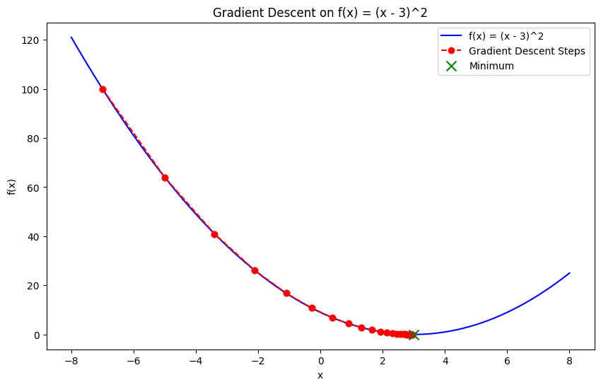
Gradient descent is one of the most fundamental techniques in numerical optimization. It is an iterative method used to find the minimum of a function by following the negative of the gradient (or slope) of the function. 

The core idea is to start with an initial guess and update it iteratively by moving toward the steepest descent until convergence is reached. It’s one of the most commonly used optimization techniques when it comes to training machine learning models, where the objective is to minimize the loss function. 

Newton's method

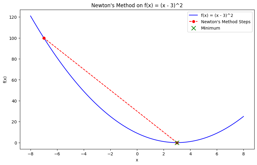
Newton's method is an optimization technique that finds the minimum using both the gradient and the second-order derivative (the Hessian matrix) of the objective function. Unlike gradient descent, which relies only on first-order derivatives, Newton’s method leverages curvature information, allowing for faster convergence, especially for convex functions.

While Newton's method converges rapidly, it requires calculating the Hessian matrix, which can be computationally expensive and impractical for large-scale problems. However, it is highly effective for small, smooth convex problems.

Conjugate gradient method

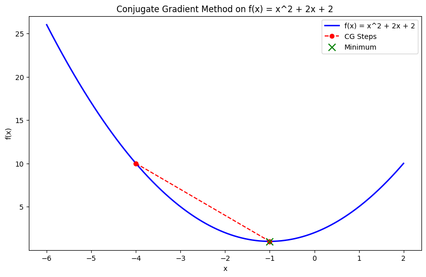
The conjugate gradient method is an efficient optimization technique used for large-scale problems, particularly where storing the Hessian matrix is impractical. It iteratively builds conjugate directions, optimizing along them rather than requiring the full Hessian, making it suitable for problems like minimizing large quadratic functions.

This method is helpful in finite element analysis or large-scale machine learning applications, where matrix computations become burdensome.

Quasi-newton methods (BFGS)

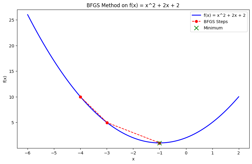
Quasi-Newton methods, like the Broyden–Fletcher–Goldfarb–Shanno (BFGS) algorithm, approximate the Hessian matrix rather than computing it directly. These methods achieve faster convergence than gradient descent by utilizing second-order information without the computational overhead of calculating the full Hessian.

Simplex method

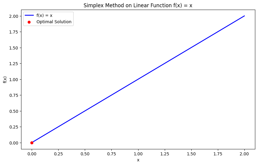
The Simplex method is a widely used algorithm for solving linear programming (LP) problems, where the objective function and constraints are linear. It systematically examines the vertices of the feasible region (a polyhedron) and moves towards the optimal vertex where the objective function reaches its maximum or minimum value.

Trust-region methods

Trust-region methods are optimization algorithms that build a local model of the objective function within a “trust region” around the current solution. 

Rather than taking steps in a predetermined direction (as in gradient descent), the algorithm defines a simpler subproblem within the trust region. It iteratively solves this subproblem to refine the solution. These methods are particularly effective for handling complex, nonlinear problems and offer better stability compared to traditional gradient-based methods.

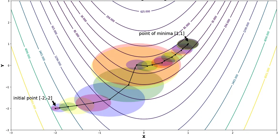
Trust regions and radii while minimizing Rosenbrock’s function | Source: Trust Region Methods by Shivangi Khare

Common Python Packages for Optimization

There are a range of libraries and packages designed to facilitate numerical optimization. Each has its strengths and applications, but regardless of the optimization problem you face, there is usually a robust tool to help you address it in Python. 

Here are four of the most common optimization packages:  

SciPy optimization (scipy.optimize)

The scipy.optimize module is a versatile library in the SciPy ecosystem, offering a wide array of algorithms for both unconstrained and constrained optimization problems. It includes functions for finding the minima of scalar and multi-variable functions, solving root-finding problems, and fitting curves to data.

Functions in this module include: 

• minimize(): A function used to minimize a scalar function of one or more variables.

from scipy.optimize import minimize

def objective_function(x):
    return x[0]**2 + x[1]**2
result = minimize(objective_function, [1, 1], method='BFGS')
print(result.x)  # Optimal solution

# >>> [-1.07505143e-08 -1.07505143e-08]

• root(): Finds the root of a vector function – extremely useful for solving systems of nonlinear equations.

from scipy.optimize import root

def equations(vars):
    x, y = vars
    return [x + 2*y - 3, x - y - 1]
result = root(equations, [0, 0])
print(result.x)

# >>> [1.66666667 0.66666667]

• curve_fit(): This function fits a curve to a set of data points and is useful for fitting data and parameter estimation.

from scipy.optimize import curve_fit
import numpy as np

def model(x, a, b):
    return a * np.exp(b * x)
x_data = np.array([1, 2, 3])
y_data = np.array([2.7, 7.4, 20.1])
params, covariance = curve_fit(model, x_data, y_data)
print(params)  # Fitted parameters

# >>> [0.9981286  1.00089935]

CVXPY

CVXPY is a Python library designed for convex optimization problems. It enables users to define and solve these problems using a high-level, declarative syntax. It simplifies formulating complex optimization problems by allowing users to specify the objective function and constraints in a natural and readable way.

CVXPY offers the following features:

• Declarative syntax: CVXPY provides an intuitive way to model optimization problems using Python's mathematical expressions.
• State-of-the-art solvers: It interfaces with advanced solvers like ECOS, SCS, and OSQP, which efficiently handle convex problems.

import cvxpy as cp

# Define variables
x = cp.Variable()
y = cp.Variable()

# Define constraints
constraints = [x + y == 1, x - y >= 2]

# Define the objective function
objective = cp.Minimize(x**2 + y**2)

# Formulate the problem
prob = cp.Problem(objective, constraints)

# Solve the problem
result = prob.solve()
print(f"Optimal value: {result}")
print(f"x: {x.value}, y: {y.value}")

# >>> Optimal value: 2.5
# x: 1.5, y: -0.5000000000000001

Pyomo

Pyomo is a flexible and comprehensive optimization modeling package that supports linear, nonlinear, and mixed-integer programming. It is designed for complex optimization problems and integrates seamlessly with solvers such as GLPK, CBC, and CPLEX.

The features of Pyomo include:

• Modeling flexibility: Pyomo allows for the definition of optimization problems with a high degree of flexibility, including complex constraints and objectives.
• Solver integration: It supports a wide range of solvers, providing flexibility in choosing the best tool for a specific problem.

Gurobi and CPLEX (via Pyomo or direct API)

Gurobi and CPLEX are high-performance solvers for large-scale optimization problems. They are commonly used in industry for tasks such as supply chain optimization, portfolio management, and logistics. 

They offer advanced algorithms designed to handle complex and large-scale problems efficiently.

• Gurobi: Accessible through Pyomo or its direct API, Gurobi is known for its speed and reliability in solving linear, integer, and quadratic programming problems.
• CPLEX: Similarly, CPLEX provides powerful optimization capabilities and is used in various sectors for solving complex operational and strategic problems. It can be accessed via Pyomo or directly through its API.

These solvers are often employed for industry-scale problems where computational efficiency and robustness are critical.

Real-World Applications of Numerical Optimization in Python

As I mentioned in the introduction, numerical optimization plays a crucial role across various domains. It provides essential techniques for solving complex problems and making data-driven decisions.

For example:  

• Machine learning: Models are fundamentally trained using numerical optimization. This involves finding the optimal parameters that minimize the loss function and quantifying how well the model predicts the target variable. 
• Operations research: Optimization techniques help make strategic decisions that maximize or minimize various operational metrics. By optimizing objective functions subject to constraints, operations researchers can improve efficiency in processes like supply chain management, workforce scheduling, and production planning. 
• Finance: Numerical optimization is crucial in the finance sector for tasks such as portfolio optimization. It helps determine the best asset allocation to maximize returns or minimize risk.
• Engineering design: Numerical optimization is applied to design systems and structures that meet specific performance criteria while minimizing costs. This process helps in achieving efficient designs for everything from bridges and aircraft to manufacturing processes and energy systems.

Best Practices for Numerical Optimization in Python

Several factors must be considered to ensure the best results from your optimization efforts in Python. Be sure to follow the following best practices: 

Choosing the correct algorithm

Selecting the right optimization algorithm is crucial for achieving optimal results. The choice of algorithm depends on the nature of the problem:

• Linear vs. nonlinear: For linear problems, linear programming techniques like the Simplex or interior-point methods are appropriate. For nonlinear problems, methods like gradient descent, Newton's method, or quasi-Newton methods (e.g., BFGS) may be more suitable.
• Constrained vs. unconstrained: For problems with constraints, algorithms such as Sequential Quadratic Programming (SQP) or methods that handle constraints natively (e.g., interior-point methods) are required. Unconstrained problems can be efficiently solved using gradient descent or Newton's method.

Choosing the correct algorithm based on the problem’s characteristics helps achieve faster convergence and more accurate solutions.

Handling constraints

Constraints in optimization problems can significantly impact the algorithm and solution strategy choice. Various approaches can be used to handle constraints:

• Penalty methods: Incorporate constraints into the objective function by adding a penalty term for constraint violations. This approach transforms a constrained problem into an unconstrained one, allowing the use of unconstrained optimization methods.
• Barrier methods: Use barrier functions to ensure that constraints are not violated. Barrier methods work by including a barrier term in the objective function that becomes infinite as the constraints are approached.
• Native support: Utilize solvers that inherently support constraints. Many modern optimization solvers, such as those available in scipy.optimize or CVXPY, are designed to handle constraints directly and efficiently.

Selecting the appropriate method for handling constraints ensures the solutions are feasible and meet all specified requirements.

Scaling and preprocessing

Proper scaling and preprocessing of data can significantly improve the performance of optimization algorithms:

• Scaling: Normalize or standardize input data to ensure features contribute equally to the objective function. This can prevent issues related to numerical stability and improve convergence rates.
• Preprocessing: Apply techniques such as feature engineering or dimensionality reduction to simplify the problem. Proper preprocessing reduces the complexity of the optimization problem and speeds up the solution process.

Interpreting results

Interpreting the results of optimization algorithms involves understanding several aspects:

• Solution quality: Evaluate the quality of the solution by checking if it satisfies the optimal conditions and constraints. Compare the results with known benchmarks or validate them using cross-validation techniques.
• Convergence criteria: Assess whether the optimization algorithm has converged by checking convergence messages, iteration counts, or changes in the objective function value. Ensure that the algorithm has reached a solution close to the true optimum.
• Numerical precision: Consider the impact of numerical precision on the results. Minor numerical errors can accumulate and affect the final solution, particularly in large-scale problems or those with tight tolerances.

Conclusion

Numerical optimization is a cornerstone of modern problem-solving. It offers powerful tools for tackling complex challenges in fields such as machine learning, engineering, finance, and operations research. 

Python's rich ecosystem of optimization libraries—such as SciPy, CVXPY, and Pyomo—makes these advanced techniques more accessible, empowering researchers, engineers, and data scientists to design efficient systems, optimize models, and make smarter, data-driven decisions. 

Armed with the right techniques and best practices, you’re now well-equipped to approach and solve even the most challenging optimization problems in Python. But check out these resources to continue your learning:

• Introduction to Optimization in Python
• Introduction to Linear Modeling in Python
• SciPy Cheat Sheet: Linear Algebra in Python
• Data Structures: A Comprehensive Guide With Python Examples