Linear Programming: Solving Real-World Optimization Problems

Operations managers face a recurring challenge: too many decisions, too many constraints, and no obvious way to find the best solution. A distribution network needs to minimize fuel costs across dozens of routes while respecting delivery windows, vehicle capacities, and driver schedules.

These two problems share a mathematical structure. When your objectives and constraints can be expressed as linear relationships, you're working with a linear programming problem. We care about linear programming because it finds optimal solutions when you're working with limited resources and competing requirements.

What makes linear programming powerful is its guarantee: if a feasible solution exists, the algorithm will find the optimal one. Of course, real-world applications rarely fit the textbook examples perfectly, but understanding the core framework helps you recognize when optimization can replace guesswork.

This guide takes you from foundations to working Python implementations. We'll progress from simple two-variable problems you can visualize geometrically to complex scenarios requiring algorithmic solutions. You'll understand both the mathematical theory that makes optimization work and the practical skills to implement solutions yourself.

What Is Linear Programming?

Linear programming optimizes a linear objective function subject to linear constraints. In a distribution routing project I worked on, the goal was to minimize total driving distance while respecting constraints like vehicle capacity and delivery time windows.

Understanding the basic structure

Every linear programming problem has three components: decision variables, an objective function, and constraints.

Decision variables represent the choices you're making. In routing problems, binary variables might indicate which vehicle visits which location. In production planning, variables might represent manufacturing quantities.

The objective function defines what you're optimizing. It must be a linear combination of your decision variables. Constraints define your problem's rules and limitations. They take three forms: equalities, less-than-or-equal, or greater-than-or-equal inequalities.

from scipy.optimize import linprog

c = [10, 15]
A_ub = [[1, 0], [0, 1]]
b_ub = [100, 80]
A_eq = [[1, 1]]
b_eq = [150]
bounds = [(0, None), (0, None)]

result = linprog(c, A_ub=A_ub, b_ub=b_ub, A_eq=A_eq, b_eq=b_eq, 
                 bounds=bounds, method='highs')

print(f"Optimal solution: Truck 1 = {result.x[0]:.1f}, Truck 2 = {result.x[1]:.1f}")
print(f"Total cost: ${result.fun:.2f}")

The code above minimizes total cost for two decision variables, subject to individual limits and a total coverage requirement. The objective coefficients [10, 15] represent cost per unit, inequality constraints limit each variable's range, and the equality constraint ensures total coverage.

Geometric interpretation

Understanding linear programming geometrically transformed how I think about optimization. Each constraint defines a half-space, and their intersection forms the feasible region. This region is always a convex polytope, meaning any line between two interior points stays inside.

Here's the crucial insight: optimal solutions always occur at vertices of the feasible region. Moving along an edge either improves your objective or doesn't, so you keep moving until hitting a corner. This property makes linear programming algorithms efficient.

import numpy as np
import matplotlib.pyplot as plt

x = np.linspace(0, 8, 400)
y1 = (10 - x) / 2
y2 = 12 - 2*x

plt.figure(figsize=(10, 8))
plt.plot(x, y1, 'r-', label='x + 2y ≤ 10', linewidth=2)
plt.plot(x, y2, 'b-', label='2x + y ≤ 12', linewidth=2)

y_feasible = np.minimum(y1, y2)
y_feasible = np.maximum(y_feasible, 0)
plt.fill_between(x, 0, y_feasible, where=(y_feasible >= 0), 
                 alpha=0.3, color='green', label='Feasible region')

vertices = [(0, 0), (0, 5), (14/3, 8/3), (6, 0)]
for v in vertices:
    plt.plot(v[0], v[1], 'ko', markersize=10)
    obj_value = 3*v[0] + 4*v[1]
    plt.annotate(f'({v[0]:.1f}, {v[1]:.1f})\nObj: {obj_value:.1f}',
                 xy=v, xytext=(v[0]+0.3, v[1]+0.3))

plt.xlim(-0.5, 8)
plt.ylim(-0.5, 8)
plt.xlabel('x')
plt.ylabel('y')
plt.legend()
plt.grid(True, alpha=0.3)
plt.title('Geometric View: Optimal Solution at Vertex (4.7, 2.7)')
plt.show()

This visualization shows the optimal solution at vertex (4.7, 2.7) where two constraints intersect. The convex feasible region guarantees no hidden valleys where algorithms might get stuck, ensuring local optima equal global optima.

Transforming real-world problems

The hardest part isn't solving the math but translating messy problems into clean formulations. Defining variables and constraints often takes more time than running the optimization itself.

Defining decision variables requires identifying fundamental choices. For routing, you might use binary variables for vehicle-location assignments, or add continuous variables for visit ordering to simplify constraints.

Constructing constraints means translating business rules into inequalities. This reveals hidden assumptions. When a manager says "each location needs one delivery," does that mean exactly one or at least one? These details change the formulation completely.

Here's an example formulation using PuLP:

from pulp import *

prob = LpProblem("Food_Bank_Routing", LpMinimize)

trucks = ['Truck_A', 'Truck_B', 'Truck_C']
centers = ['North', 'South', 'East', 'West', 'Central']

x = LpVariable.dicts("route", 
                     [(i, j) for i in trucks for j in centers],
                     cat='Binary')

distances = {
    ('Truck_A', 'North'): 15, ('Truck_A', 'South'): 20,
    ('Truck_A', 'East'): 10, ('Truck_A', 'West'): 25,
    ('Truck_A', 'Central'): 5,
    ('Truck_B', 'North'): 18, ('Truck_B', 'South'): 15,
    ('Truck_B', 'East'): 12, ('Truck_B', 'West'): 22,
    ('Truck_B', 'Central'): 8,
    ('Truck_C', 'North'): 20, ('Truck_C', 'South'): 25,
    ('Truck_C', 'East'): 15, ('Truck_C', 'West'): 18,
    ('Truck_C', 'Central'): 10,
}

prob += lpSum([distances[i, j] * x[i, j] 
               for i in trucks for j in centers])

for j in centers:
    prob += lpSum([x[i, j] for i in trucks]) == 1

max_stops = {'Truck_A': 3, 'Truck_B': 2, 'Truck_C': 3}
for i in trucks:
    prob += lpSum([x[i, j] for j in centers]) <= max_stops[i]

prob.solve()

print(f"Status: {LpStatus[prob.status]}")
print(f"Total distance: {value(prob.objective)} miles")
for i in trucks:
    route = [j for j in centers if value(x[i, j]) == 1]
    print(f"{i} visits: {', '.join(route)}")

The formulation above uses binary variables for truck-center assignments, minimizes total distance, ensures each center gets exactly one delivery, and respects truck capacity limits.

Classic problem patterns provide templates. The diet problem minimizes cost while meeting nutrition requirements. Transportation problems minimize shipping costs. This one directly applied to my own routing challenge. Recognizing these patterns accelerates formulation since you're rarely solving truly novel problems.

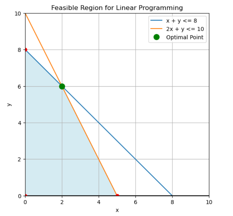
Linear programming finds optimal solutions at the vertices of feasible regions defined by constraints. Image by Author

Solution Methods and Algorithmic Approaches

Understanding how algorithms work changed my appreciation for calling linprog(). These aren't black boxes but elegant mathematical procedures.

Simplex algorithm

The simplex algorithm, developed by George Dantzig in 1947, is the starting point. Its insight: systematically traverse from vertex to adjacent vertex, always improving the objective, until reaching the optimum.

The algorithm maintains a tableau and performs pivot operations to move between vertices. Each iteration improves the objective or determines optimality by selecting a pivot element and updating through row operations.

from scipy.optimize import linprog
import numpy as np

c = [-3, -2]
A_ub = [[2, 1], [2, 3], [3, 1]]
b_ub = [18, 42, 24]
bounds = [(0, None), (0, None)]

result = linprog(c, A_ub=A_ub, b_ub=b_ub, bounds=bounds, method='highs')

print(f"Optimal solution: x1 = {result.x[0]:.2f}, x2 = {result.x[1]:.2f}")
print(f"Maximum value: {-result.fun:.2f}")
print(f"Iterations: {result.nit}")

The code above demonstrates solving a maximization problem with the simplex method by negating the objective coefficients. The solver systematically moves between vertices of the feasible region defined by the constraints, reaching the optimal solution in just a few iterations. In larger problems, the simplex method can find the optimum in far fewer steps than the number of feasible vertices, often under 20 iterations even with thousands of possibilities.

Interior-point methods

While simplex traverses boundaries, interior-point methods navigate through the feasible region's interior. For large portfolio optimization problems with hundreds of assets, simplex can become sluggish while interior-point methods solve in seconds.

The key advantage is polynomial-time complexity. Karmarkar's algorithm (1984) made interior-point methods practical, balancing objective improvement with staying far from constraint boundaries. Modern solvers like Gurobi automatically select between simplex and interior-point based on problem characteristics.

Graphical method for two variables

For two-variable problems, I always solve them graphically first. This builds intuition that transfers to higher dimensions. Plot constraints, identify the feasible region, and find which corner optimizes the objective.

from scipy.optimize import linprog

c = [-30, -40]
A_ub = [[2, 1], [1, 2]]
b_ub = [100, 80]
bounds = [(0, None), (0, None)]

result = linprog(c, A_ub=A_ub, b_ub=b_ub, bounds=bounds, method='highs')

print(f"Bread loaves: {result.x[0]:.0f}")
print(f"Cakes: {result.x[1]:.0f}")
print(f"Maximum profit: ${-result.fun:.0f}")

This bakery production problem maximizes profit from bread and cakes, subject to oven and decoration hour limits. The solution reveals which corner point is optimal geometrically, making the algorithm's vertex-hopping behavior concrete.

Applications Across Industries

Linear programming applies the same mathematical framework to solve problems across wildly different domains.

Manufacturing and production

Production planning was my first serious application. The production mix problem determines manufacturing quantities, with variables representing production, objectives maximizing profit, and constraints capturing resource limitations.

from pulp import *

products = ['Phone', 'Tablet', 'Laptop']

profits = {'Phone': 120, 'Tablet': 200, 'Laptop': 350}
assembly_time = {'Phone': 2, 'Tablet': 3, 'Laptop': 5}
testing_time = {'Phone': 1, 'Tablet': 1.5, 'Laptop': 2}

assembly_available = 500
testing_available = 200
min_production = {'Phone': 50, 'Tablet': 30, 'Laptop': 20}

model = LpProblem("Production_Planning", LpMaximize)
production = LpVariable.dicts("produce", products, lowBound=0, cat='Integer')

model += lpSum([profits[p] * production[p] for p in products])
model += lpSum([assembly_time[p] * production[p] for p in products]) <= assembly_available
model += lpSum([testing_time[p] * production[p] for p in products]) <= testing_available

for p in products:
    model += production[p] >= min_production[p]

model.solve()

print(f"Status: {LpStatus[model.status]}")
for p in products:
    print(f"{p}: {production[p].varValue:.0f} units")
print(f"Total profit: ${value(model.objective):,.0f}")

The model above optimizes electronics production across three product lines, balancing assembly and testing capacity with minimum production requirements.

Blending problems optimize mixtures meeting specifications at minimum cost, such as blending food items to meet nutritional requirements while minimizing cost.

Transportation and logistics

The transportation problem is another studied example. The classical structure has sources with supplies and destinations with demands, minimizing total shipping cost.

warehouses = ['Warehouse_A', 'Warehouse_B', 'Warehouse_C']
supply = {'Warehouse_A': 300, 'Warehouse_B': 400, 'Warehouse_C': 200}

customers = ['Customer_1', 'Customer_2', 'Customer_3', 'Customer_4']
demand = {'Customer_1': 200, 'Customer_2': 150, 'Customer_3': 250, 'Customer_4': 200}

costs = {
    ('Warehouse_A', 'Customer_1'): 8,  ('Warehouse_A', 'Customer_2'): 6,
    ('Warehouse_A', 'Customer_3'): 10, ('Warehouse_A', 'Customer_4'): 7,
    ('Warehouse_B', 'Customer_1'): 9,  ('Warehouse_B', 'Customer_2'): 12,
    ('Warehouse_B', 'Customer_3'): 8,  ('Warehouse_B', 'Customer_4'): 11,
    ('Warehouse_C', 'Customer_1'): 14, ('Warehouse_C', 'Customer_2'): 7,
    ('Warehouse_C', 'Customer_3'): 10, ('Warehouse_C', 'Customer_4'): 12,
}

model = LpProblem("Transportation", LpMinimize)

routes = [(w, c) for w in warehouses for c in customers]
shipments = LpVariable.dicts("ship", routes, lowBound=0)

model += lpSum([costs[i, j] * shipments[i, j] for (i, j) in routes])

for w in warehouses:
    model += lpSum([shipments[w, c] for c in customers]) <= supply[w]

for c in customers:
    model += lpSum([shipments[w, c] for w in warehouses]) >= demand[c]

model.solve()

Network flow problems generalize transportation to graphs with transshipment nodes. I've read that airlines use this extensively for crew scheduling and aircraft routing.

Financial services and healthcare

In financial applications, capital budgeting selects projects maximizing return subject to budget constraints:

projects = {
    'Project_A': {'return': 25000, 'cost': 100000, 'staff': 5},
    'Project_B': {'return': 30000, 'cost': 150000, 'staff': 7},
    'Project_C': {'return': 20000, 'cost': 80000, 'staff': 4},
}

budget = 300000
staff_available = 15

model = LpProblem("Capital_Budgeting", LpMaximize)
select = LpVariable.dicts("select", projects.keys(), cat='Binary')

model += lpSum([projects[p]['return'] * select[p] for p in projects])
model += lpSum([projects[p]['cost'] * select[p] for p in projects]) <= budget
model += lpSum([projects[p]['staff'] * select[p] for p in projects]) <= staff_available

model.solve()

Healthcare systems face endless optimization challenges. I consulted on a clinic scheduling problem that assigned nurses to shifts while respecting skill requirements and workload balance.

Modern technology applications

Linear programming also appears unexpectedly within machine learning. Feature selection can be formulated as minimizing prediction error subject to sparsity constraints. Cloud computing uses it for resource allocation across distributed systems.

Computational Complexity and Performance

Complexity matters when problems scale from toy examples to production systems.

Simplex algorithm complexity

Simplex has a fascinating level of complexity. It has an exponential worst-case but excellent average-case performance. Pathological cases like the Klee-Minty cube force it to examine every vertex, but typical problems examine only a small fraction, scaling roughly quadratically.

I tested this by solving randomly generated problems of increasing size:

import time
import numpy as np
from scipy.optimize import linprog

def benchmark_simplex(num_vars, num_constraints):
    c = np.random.randn(num_vars)
    A_ub = np.random.randn(num_constraints, num_vars)
    b_ub = np.random.rand(num_constraints) * 10
    
    start = time.time()
    result = linprog(c, A_ub=A_ub, b_ub=b_ub, method='simplex')
    elapsed = time.time() - start
    
    return elapsed, result.nit

problem_sizes = [(10, 20), (50, 100), (100, 200), (200, 400)]

for n_vars, n_const in problem_sizes:
    times, iterations = [], []
    for _ in range(10):
        t, it = benchmark_simplex(n_vars, n_const)
        times.append(t)
        iterations.append(it)
    print(f"{n_vars}x{n_const}: {np.mean(times):.4f}s, {np.mean(iterations):.1f} iterations")

My benchmarks showed doubling problem size increased time by less than 4x, confirming near-polynomial behavior for typical distributions.

Performance improvements

Modern solvers achieve remarkable performance through preprocessing, parallel processing, and automatic algorithm selection. Preprocessing can reduce problem size by 30% or more automatically before solving.

Degeneracy occurs when multiple constraints are tight at the optimum, potentially causing cycling. I encountered this when two routes had identical costs. Solvers use perturbation techniques to avoid cycling, though degenerate problems solve more slowly.

Numerical instability arises with poorly scaled problems. Mixing monetary amounts (thousands of dollars) with quantities (single units) caused solver warnings. Rescaling fixed it immediately.

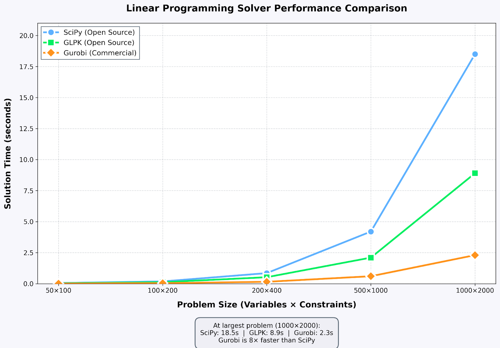
Solver performance comparison: commercial solutions excel on large-scale problems. Image by Author

Software Tools and Implementation

Tool choice dramatically impacts productivity. I've progressed from hand-coding simplex to using professional solvers handling vastly larger problems.

Commercial solvers and modeling languages

CPLEX and Gurobi dominate industrial optimization, offering order-of-magnitude better performance than open-source alternatives for large problems. I used Gurobi's academic license for supply chain work. Problems taking minutes with SciPy solved in seconds.

PuLP is my Python go-to. It provides a clean API for formulating models solved by various backends:

from pulp import *

model = LpProblem("my_problem", LpMaximize)

x = LpVariable("x", lowBound=0)
y = LpVariable("y", lowBound=0)

model += 3*x + 2*y
model += x + y <= 100
model += 2*x + y <= 150

model.solve()

print(f"Used solver: {model.solver}")
print(f"Status: {LpStatus[model.status]}")

The abstraction layer means solver-agnostic code that runs on different systems. Pyomo offers more advanced features for complex optimization, including nonlinear and stochastic programming.

Cloud and open-source alternatives

Cloud platforms offer optimization-as-a-service for irregular large-scale problems. You upload problem data and receive solutions via API. The serverless architecture is elegant though slower than local solvers for small problems.

GLPK (GNU Linear Programming Kit) is the reliable open-source workhorse. I use it for teaching and personal projects. HiGHS is a newer solver showing impressive performance. SciPy recently adopted HiGHS as its default backend, and my benchmarks showed it matching Gurobi on many problems.

Linear Programming Examples

Working through complete examples builds understanding better than theory alone.

Example 1: Diet problem

The classic diet problem minimizes cost while meeting nutritional requirements:

from pulp import *

foods = {
    'Oatmeal': {'cost': 0.50, 'calories': 110, 'protein': 4, 'vitamin': 2},
    'Chicken': {'cost': 2.50, 'calories': 250, 'protein': 30, 'vitamin': 0},
    'Eggs':    {'cost': 0.80, 'calories': 155, 'protein': 13, 'vitamin': 1},
    'Milk':    {'cost': 1.20, 'calories': 150, 'protein': 8, 'vitamin': 4},
    'Bread':   {'cost': 0.30, 'calories': 80, 'protein': 3, 'vitamin': 0}
}

min_calories, min_protein, min_vitamin = 2000, 50, 10

model = LpProblem("Diet_Optimization", LpMinimize)
servings = LpVariable.dicts("servings", foods.keys(), lowBound=0)

model += lpSum([foods[f]['cost'] * servings[f] for f in foods])
model += lpSum([foods[f]['calories'] * servings[f] for f in foods]) >= min_calories
model += lpSum([foods[f]['protein'] * servings[f] for f in foods]) >= min_protein
model += lpSum([foods[f]['vitamin'] * servings[f] for f in foods]) >= min_vitamin

model.solve()

print(f"Total cost: ${value(model.objective):.2f}")
for food in foods:
    if servings[food].varValue > 0.01:
        print(f"{food}: {servings[food].varValue:.2f} servings")

The formulation above finds the cheapest combination of foods meeting daily nutritional requirements. This demonstrates that optimal LP solutions aren't always practical without additional constraints for variety, taste, or dietary preferences.

This same framework can also serve as a foundation for business decisions like optimizing production schedules or allocating marketing budgets.

Example 2: Multiperiod planning

Multiperiod planning considers how inventory levels affect future needs across multiple time periods:

days = ['Monday', 'Tuesday', 'Wednesday', 'Thursday', 'Friday']

centers = {
    'North': {'daily_demand': [100, 80, 90, 110, 85], 'capacity': 250},
    'South': {'daily_demand': [120, 100, 95, 105, 130], 'capacity': 300},
}

delivery_cost = {'Monday': 50, 'Tuesday': 50, 'Wednesday': 50,
                 'Thursday': 50, 'Friday': 70}

model = LpProblem("Multiperiod_Routing", LpMinimize)

deliveries = LpVariable.dicts("deliver",
                              [(c, d) for c in centers for d in days],
                              lowBound=0)
inventory = LpVariable.dicts("inventory",
                            [(c, d) for c in centers for d in days],
                            lowBound=0)

model += lpSum([delivery_cost[d] * deliveries[c, d] 
                for c in centers for d in days])

for c in centers:
    for i, day in enumerate(days):
        if i == 0:
            model += inventory[c, day] == deliveries[c, day] - centers[c]['daily_demand'][i]
        else:
            prev_day = days[i-1]
            model += (inventory[c, day] == inventory[c, prev_day] + 
                     deliveries[c, day] - centers[c]['daily_demand'][i])
        model += inventory[c, day] <= centers[c]['capacity']

model.solve()

Multiperiod models increase problem size but unlock sophisticated optimization. The model consolidates deliveries on cheaper days, using storage capacity to reduce overall costs.

Mixed-Integer Programming

Many problems involve discrete decisions: build a facility or don't, assign a worker or don't. This requires mixed-integer programming (MIP), extending linear programming with integer and binary variables.

Introduction and branch-and-bound

Routing problems need integer decisions. The binary variable x[i][j] indicates whether vehicle i visits location j. Vehicles can't make fractional visits.

Branch-and-bound systematically searches a discrete solution space by solving continuous LP relaxations:

from pulp import *

model_continuous = LpProblem("Continuous", LpMaximize)
x_cont = LpVariable("x", lowBound=0)
y_cont = LpVariable("y", lowBound=0)

model_continuous += 3*x_cont + 4*y_cont
model_continuous += x_cont + 2*y_cont <= 10
model_continuous += 2*x_cont + y_cont <= 12

model_continuous.solve()
print(f"Continuous: x={x_cont.varValue:.2f}, y={y_cont.varValue:.2f}")

model_integer = LpProblem("Integer", LpMaximize)
x_int = LpVariable("x", lowBound=0, cat='Integer')
y_int = LpVariable("y", lowBound=0, cat='Integer')

model_integer += 3*x_int + 4*y_int
model_integer += x_int + 2*y_int <= 10
model_integer += 2*x_int + y_int <= 12

model_integer.solve()
print(f"Integer: x={x_int.varValue:.0f}, y={y_int.varValue:.0f}")

The integer solution differs from rounding the continuous solution. Branch-and-bound finds the optimal integer solution, but at significantly higher computational cost.

When to use integer programming

Use integer variables when decisions are inherently discrete: opening facilities, assigning workers, routing vehicles. Optimizations in the bond market often require mixed integer solutions. Continuous variables can produce nonsensical fractional assignments, while binary variables yield implementable solutions.

However, integer programming is dramatically more expensive. Problems with hundreds of integer variables can take hours versus seconds for continuous LPs. If production quantities are large, integrality matters less since rounding barely affects solutions. Always solve the continuous relaxation first to check bounds before committing to full integer programming.

Conclusion

Linear programming transforms how you approach optimization problems. The same mathematical framework applies across drastically different domains, from routing to production planning to portfolio management.

Start with simple two-variable problems you can visualize geometrically. Implement basic simplex to understand what commercial solvers do behind the scenes. Work with real formulations, translating business requirements into mathematical constraints.

To deepen your expertise, explore our Introduction to Optimization in Python and Linear Algebra for Data Science courses to strengthen your mathematical foundations. Our Machine Learning Scientist in Python career track is another great option.