Course
Data Analysis in Excel
3 hr
140.7K
It usually happens at the worst time: a spreadsheet that worked fine yesterday suddenly throws a circular reference warning right before a deadline.
The good news? These circular references are easier to fix than you think.
In this guide, I’ll explain:
A circular reference in Excel happens when a formula refers back to its own cell (directly or indirectly) and creates a calculation loop that Excel can’t resolve. For example, if cell A1 contains =A1+10, Excel keeps trying to calculate the result forever.
Even indirect loops cause trouble. If A1 depends on B1, B1 depends on C1, and C1 depends on A1, Excel is stuck. The file may take a long time to calculate, display incorrect values, or stop updating entirely.
Now, some circular references are simple formula mistakes, while others are intentional design choices used in advanced models. I'll get to that distinction later on, but first explore the different types.
A direct circular reference occurs when a formula includes its own cell address. Suppose you have two values in cells A2 and B2. If in cell C2 we type A2 + B2 + C2, C2 is referencing itself directly.
When you enter the formula and press Enter, a circular reference pop-up appears. And when you click OK, the formula returns an unexpected result of some kind.
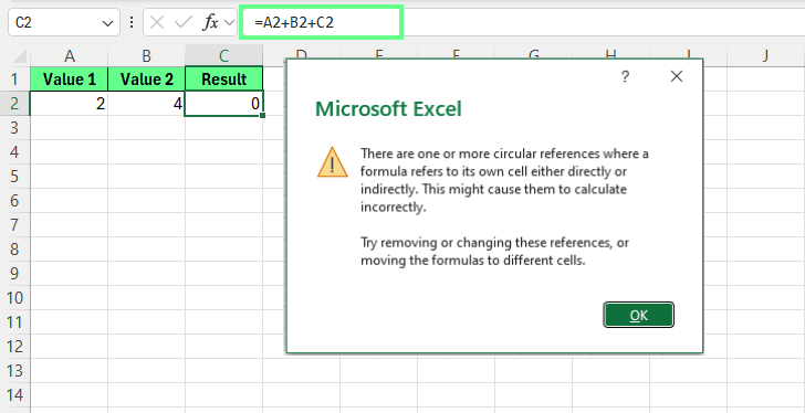
Direct circular reference. Image by Author.
This returns 0 because when we add A2 and B2, it should return 6, but 'C2' keeps adding itself. Excel cannot calculate C2 without knowing the value of C2. This creates an immediate loop that never resolves.
Note: These circular references are the easiest to identify because the self-reference is visible directly in the formula syntax. In fact, Excel detects and flags them as soon as the formula is entered.
An indirect circular reference occurs when multiple cells form a dependency chain that loops back to the starting point.
For example:
F2 references H4
H4 references E4
E4 references F2
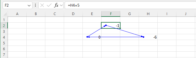
Indirect circular reference. Image by Author.
No single formula looks wrong on its own. The problem only appears when Excel traces the entire chain and realizes the calculation returns to where it started.
These are harder to detect because the loop can span many cells and, in complex workbooks, even multiple worksheets, before Excel identifies the circular dependency.
A hidden circular reference is one where the dependency loop isn’t obvious from the formula syntax. These often come from:
Named ranges
INDIRECT() or OFFSET() functions
Complex conditional logic
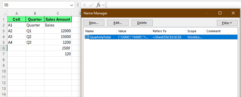
For example, a named range QuarterlyTotal includes cells C3 through C5, which contain quarterly sales values.
In cell C5, the formula bar shows:
=QuarterlyTotal*0.1At first glance, this looks fine. The formula doesn’t reference C5 directly. However, because QuarterlyTotal includes C5, Excel must calculate C5 as part of the total used to calculate C5.
This creates a hidden loop:
Excel tries to calculate QuarterlyTotal
QuarterlyTotal includes C5
C5 depends on QuarterlyTotal
The reference is circular, even though the formula syntax doesn’t show it explicitly.
This is what makes hidden circular references so difficult to troubleshoot. The formulas appear correct, the workbook may calculate normally for a long time, and the circular reference only surfaces when Excel evaluates the named range.
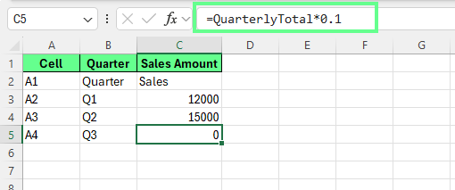
Hidden circular reference. Image by Author.
Conditional logic can make this even harder to detect. Why? Because nested IF() statements may only create a circular reference under specific conditions. As a result, the file works until certain values change.
Hidden circular references are the most challenging to fix because the dependency loop is concealed by abstraction rather than by visible cell references.
Some circular references exist by design. Others are errors you need to eliminate.
An intentional circular reference is created on purpose to support specific modeling needs where values depend on each other.
Take financial modeling as an example: interest expense depends on the outstanding debt balance, while the debt balance changes based on cash flow, which includes interest expense. This creates a feedback loop that reflects real-world business logic.
The model starts with a simple structure:
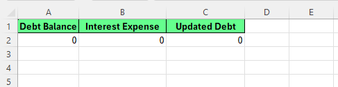
Intentional circular references. Image by Author.
When interest is calculated based on debt, and the updated debt includes that interest, the calculation naturally loops back on itself. Excel flags this as a circular reference and returns zero by default because it cannot resolve the dependency in a single pass.
To prevent this, turn on iterative calculation like this:
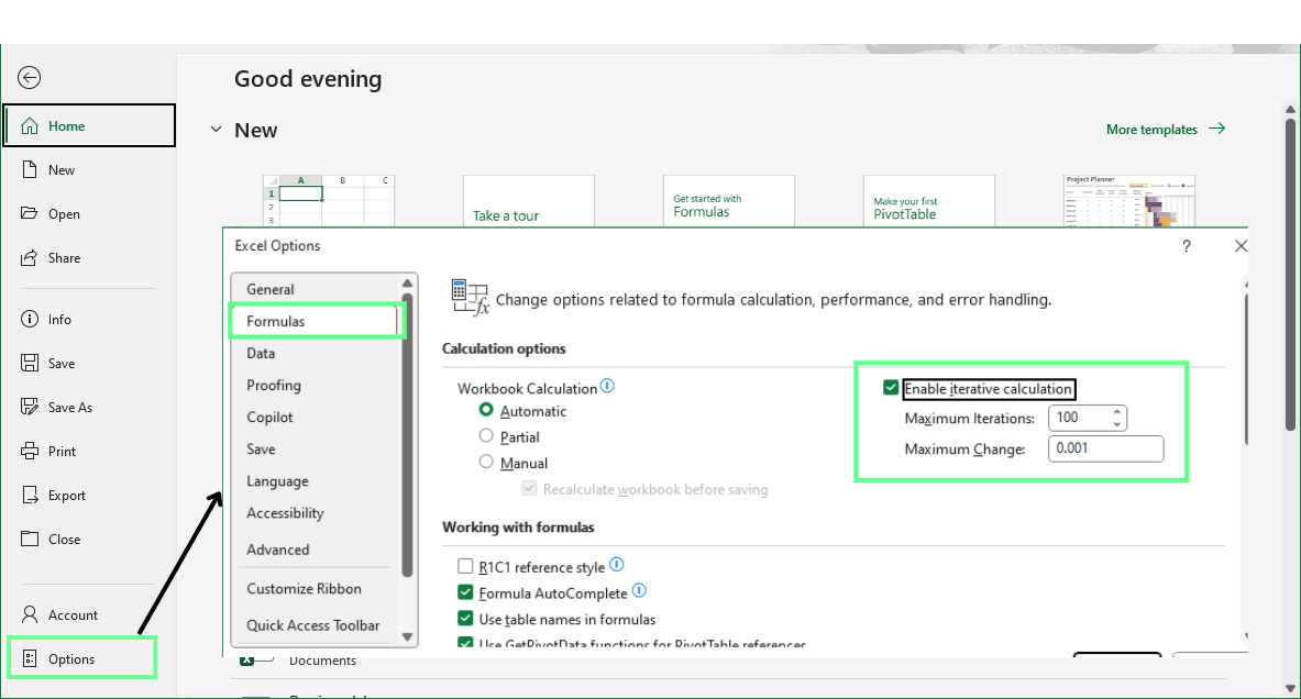
Enable the iterative calculation option. Image by Author.
Once iterative calculation is enabled, Excel repeatedly recalculates the interest and updated debt values. With each pass, the numbers adjust slightly until they stabilize and stop changing.
The final result represents a converged solution rather than a single-step calculation. This works because the circular reference is intentional. Interest affects debt, and debt affects interest. Each value influences the other, so repeated recalculation is expected and necessary.
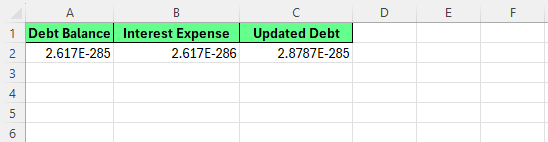
Iterative calculation. Image by Author.
Note: Iterative calculation does not guarantee a meaningful result on its own. It repeats the logic you have built into the model, which is why intentional circular references require careful monitoring and validation.
An accidental circular reference results from formula errors, copy-paste mistakes, or unintended changes. Suppose you enter values 2, 4, and 6 in cells A1:A3.
In A4, you want a total, so you enter:
=SUM(A1:A4)Cell A4 now includes itself in the calculation.
When you press Enter, Excel shows a circular reference warning. After clicking OK, Excel returns 0.
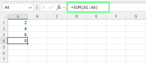
Accidental circular reference. Image by Author.
This circular reference does not represent real logic. It exists because the formula range is wrong.
Once Excel flags a loop, you now have to locate exactly where it starts and decide how to resolve it.
Let’s look at a few methods to fix circular references, depending on whether it is accidental or intentional:
Excel includes several built-in detection tools to quickly pinpoint circular references, each with its own strengths and limitations. Let’s walk through these options.
The fastest way to detect a circular reference is through the status bar at the bottom-left corner of the Excel window.
When a circular reference exists, Excel displays text such as “Circular References: G4.” This tells you the most recently detected cell involved in a loop.
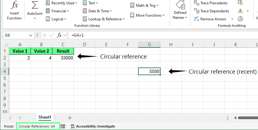
Display circular reference on the status bar. Image by Author.
However, the status bar shows only one circular reference at a time. If multiple loops exist, Excel reveals them one by one.
Here’s how to fix this:
Tip: Write down each cell address, because fixing one loop often reveals another.
Excel also displays a warning message when:
The warning usually states that one or more formulas refer to themselves and may calculate incorrectly.
These warnings may stop appearing if:
If the results look incorrect and no warning appears, force a recalculation like this:
Tip: Closing and reopening the workbook can also cause Excel to display the warning again.
To view multiple circular references at once, use Excel’s Error Checking tool: Go to Formulas > Error Checking > Circular References
This menu lists all detected circular references and lets you jump directly to each cell, which makes it easier to diagnose complex workbooks.
If the Circular References submenu appears empty but Excel is still behaving incorrectly, press F9 to force recalculation and refresh the list.
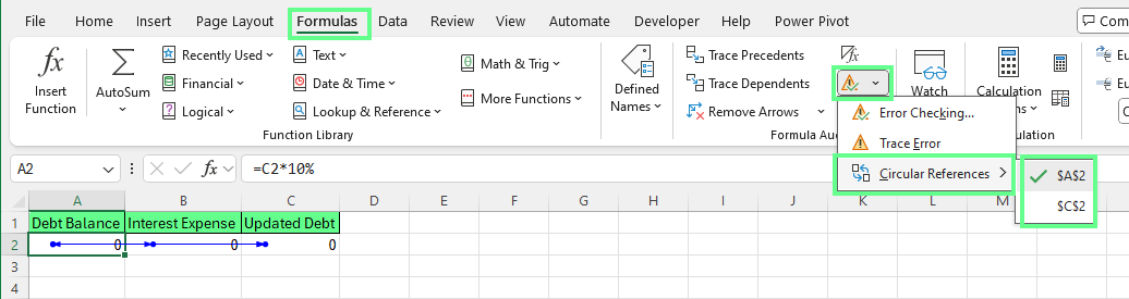
An error-checking tool to find circular references. Image by Author.
Note: In Excel 2007 and later, this feature is available in the Ribbon. Older versions surface similar options through the menu bar.
Once you’ve identified a problematic cell, use visual tracing tools to see how the circular reference forms.
These tools draw arrows between cells and make dependencies visible instead of hidden inside formulas. Both are available in the Formula Auditing group on the Formulas tab:
If tracing precedents and dependents eventually leads back to the starting cell, the arrows form a loop and confirm the circular reference.
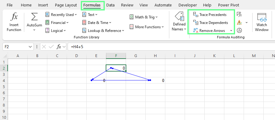
Trace Precedents and Trace Dependents. Image by Author.
After correcting the formula, the arrows no longer loop back, and the circular reference disappears. You can remove the arrows using Remove Arrows in the same menu.
Most circular references occur because calculations are ordered incorrectly, not because Excel is malfunctioning. For such accidental circular references, formula restructuring is the most effective solution.
Here are a few methods to fix this:
Circular references often appear when a formula tries to calculate a value using its own result.
For example, a formula like =A2+1 in cell A2 creates an immediate loop because the cell depends on itself. To fix this, move the required input to a separate cell and reference that value instead.
Once the dependency is removed, Excel can calculate the formula normally.
Circular references also occur when a single formula tries to handle multiple steps at once.
For example, if two cells depend on each other to calculate a shared value, Excel has no clear starting point. To fix this, introduce a helper cell that performs the intermediate calculation first.
By calculating shared values in a separate helper cell, Excel can follow a clear order:
This approach simplifies formulas and eliminates circular dependencies.
Totals and summary formulas should not be mixed into the same cells they depend on. When a summary pulls numbers from a range that includes itself, Excel creates a circular reference.
For example, if A2 contains a base amount of 1000, and B2 contains a rate of 10%, C2 displays the total amount, and D2 calculates a fee.
If C2 uses =A2+D2 and D2 uses this =C2*$B$2, a circular reference appears because the total depends on the fee, and the fee depends on the total.
Excel cannot calculate either one first.
To fix this, the fee should be calculated from the base value, not from the total. So change D2 to =A2*$B$2 and keep C2 as =A2+D2.
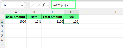
Use separate cells to avoid circular reference. Image by Author.
Now Excel can calculate the fee first and then add it to the base value. The circular reference disappears because each formula has a clear starting point.
Iterative calculation should be used only when circular references are intentional design elements, not accidental errors. This method is appropriate for financial models and other scenarios where legitimate feedback loops exist, and the circular logic reflects real-world behavior.
To enable iterative calculation in Excel for Windows:
Once enabled, Excel repeatedly recalculates formulas involved in circular references until they stabilize or reach a stopping condition.
Two settings control how iterative calculation behaves:
Increasing either setting can improve precision but may slow down recalculation in large workbooks.
Enable iterative calculation only when:
This method is not a fix for accidental circular references caused by formula errors.
Before enabling iterative calculation, keep these risks in mind:
Because of these risks, iterative calculation should always be explicitly documented.
A circuit breaker is an advanced technique that gives you control over when circular logic is active. Instead of removing a circular reference, you deliberately pause or allow it using a control value inside the formula.
This approach is best suited for financial modelers and power users who need circular logic in some scenarios but not all the time.
A circuit breaker typically uses:
A control cell (often set to 0 or 1)
An IF statement that switches between circular and non-circular logic
The general pattern looks like this:
=IF($A$1=1, circular_logic, non_circular_alternative)0, the formula avoids the circular reference1, the circular logic is allowed to runLet’s say you enter the following values:
A1: Circuit breaker (0 or 1)
A2: Starting balance = 1000
B2: Interest
C2: Updated balance
In B2, use =IF($A$1=1, C2*10%, A2*10%) and in C2 enter =A2+B2
Now:
When A1 = 0, interest is calculated from the starting balance. The circular reference is disabled, and Excel calculates normally.
When A1 = 1, interest is calculated from the updated balance. The circular logic becomes active and creates an intentional feedback loop.
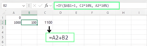
Using a circuit breaker. Image by Author.
Circuit breakers are helpful for:
This is the nuclear option: use it when other methods fail. It’s appropriate for workbooks with hopelessly tangled dependencies, inherited files with unclear logic, or situations where time pressure demands a fast yet reliable solution.
Instead of trying to untangle broken formulas, you reset the model and rebuild it methodically.
Let’s see how.
Before making any changes, create a full backup of the workbook. To do so:
Open the workbook in Excel
Go to File > Save As > Browse and choose a different location or keep the same folder to save your file
Rename the file, for example, Workbook_Backup.xlsx
Click Save
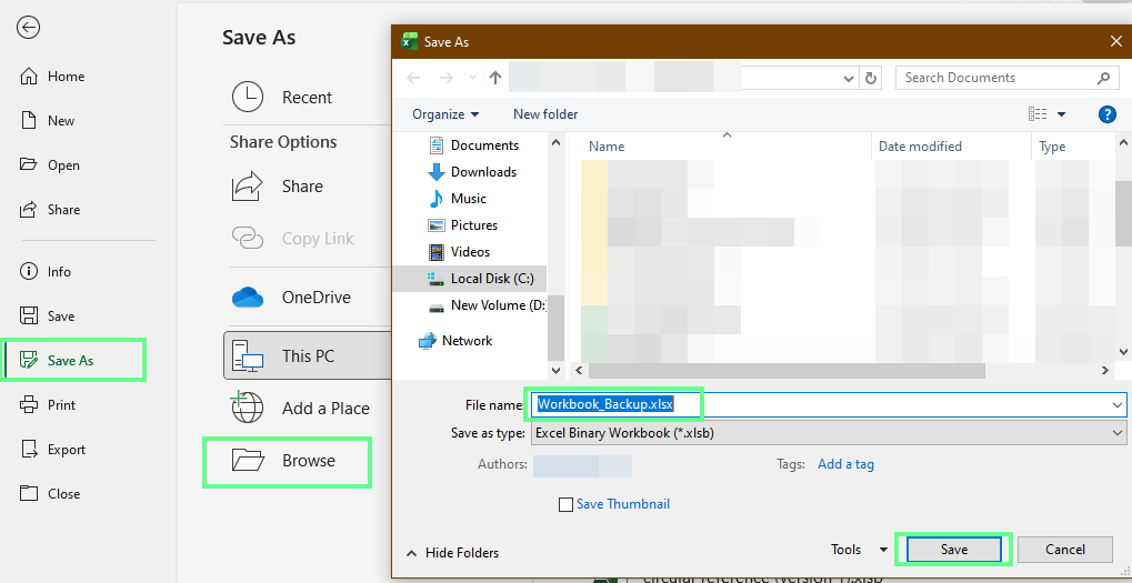
Create a backup copy of a workbook. Image by Author.
This preserves the original formulas, logic, and results so you can reference them later or roll back if needed.
Never attempt this method on the only copy of a file.
Next, capture how the workbook currently works:
This documentation helps you understand what needs to be rebuilt and prevents important logic from being lost during cleanup.
To break all circular dependencies at once, copy affected ranges and use Paste Special. Right-click > Paste Special > Values to replace formulas with their calculated results.
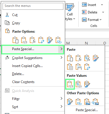
Use the Paste Special option. Image by Author.
This removes every circular reference immediately while preserving the visible numbers as a temporary baseline.
Rebuild the workbook section by section instead of all at once:
As each section is rebuilt, compare the results with the backup file. You may notice differences that indicate:
Some circular references don’t show up using Excel’s standard tools. In such cases, try advanced techniques:
When manual tracing is too slow, VBA can scan thousands of cells in seconds and identify circular references across the entire workbook.
The basic approach looks like this:
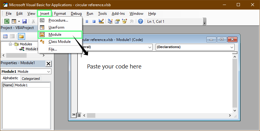
VBA interface. Image by Author.
Tip: You don’t need to write VBA from scratch. Describe what you want in plain language and let ChatGPT generate a custom detection macro.
Here’s an example VBA script:
Option Explicit
Public Sub HighlightCircularReferences_ActiveSheet()
    Dim ws As Worksheet, c As Range
    Dim hasAny As Boolean

    Set ws = ActiveSheet

    Application.ScreenUpdating = False

    ' Optional: clear previous highlighting (only on used range)
    On Error Resume Next
    ws.UsedRange.Interior.Pattern = xlNone
    On Error GoTo 0

    ' Scan formula cells only
    On Error Resume Next
    For Each c In ws.UsedRange.SpecialCells(xlCellTypeFormulas)
        On Error GoTo 0

        If IsCircularFormula(c) Then
            c.Interior.Color = RGB(255, 230, 153) ' light yellow
            hasAny = True
        End If
    Next c

    Application.ScreenUpdating = True

    If hasAny Then
        MsgBox "Circular reference cells highlighted on: " & ws.Name, vbInformation
    Else
        MsgBox "No circular references found on: " & ws.Name, vbInformation
    End If
End Sub

Private Function IsCircularFormula(ByVal startCell As Range) As Boolean
    Dim inPath As Object
    Set inPath = CreateObject("Scripting.Dictionary")

    IsCircularFormula = TraceForCycle(startCell, startCell, inPath, 0)
End Function

Private Function TraceForCycle(ByVal startCell As Range, ByVal curCell As Range, _
                               ByVal inPath As Object, ByVal depth As Long) As Boolean
    Dim prec As Range, a As Range, x As Range
    Dim key As String

    ' Safety limit to avoid deep/huge graphs freezing Excel
    If depth > 200 Then Exit Function

    key = curCell.Parent.Name & "!" & curCell.Address(False, False)

    If inPath.Exists(key) Then
        ' We hit a loop in the current path
        TraceForCycle = True
        Exit Function
    End If

    inPath.Add key, True

    ' Direct precedents (cells referenced by curCell)
    On Error Resume Next
    Set prec = curCell.DirectPrecedents
    On Error GoTo 0

    If Not prec Is Nothing Then
        For Each a In prec.Areas
            For Each x In a.Cells
                ' If any precedent is the start cell -> circular
                If x.Address(External:=True) = startCell.Address(External:=True) Then
                    TraceForCycle = True
                    Exit Function
                End If

                ' Recurse only within worksheets (avoid names/constants)
                If x.Parent Is curCell.Parent Or True Then
                    If TraceForCycle(startCell, x, inPath, depth + 1) Then
                        TraceForCycle = True
                        Exit Function
                    End If
                End If
            Next x
        Next a
    End If

    inPath.Remove key
End Function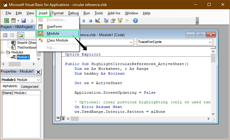
Use VBA macros to identify the cells with circular references. Image by Author.
This macro checks the active sheet for circular references in formulas. If a formula refers back to itself, directly or through other cells, the macro highlights those cells so you can easily see where the problem is. This works even if the Iterative calculation is ON.
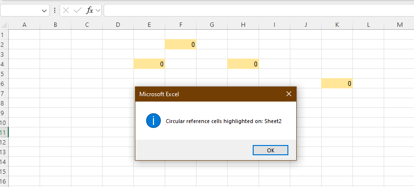
VBA highlighted the circular reference cells. Image by Author.
Circular references that span multiple worksheets are harder to detect because trace arrows don’t cross tabs.
It may look like this:
One way to detect this is to map sheet dependencies. To do so, write down which sheets reference other sheets and look for loops in that list.
You can also use Find & Replace to locate cross-sheet references:
Press Ctrl + H
Enter a sheet name followed by ! (for example, Sheet1!)
Click Find All
Excel will list every formula that references that sheet, so you can trace cross-tab dependencies.
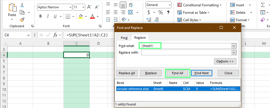
Find the connected sheets in a workbook. Image by Author.
Note: Find & Replace does not detect circular references automatically. It only locates cross-sheet dependencies, which you then analyze for loops.
Named ranges can hide circular references because formulas no longer show direct cell addresses. To review them:
Check the named ranges. Image by Author.
Some circular references only appear under specific conditions.
For example:
=IF(A1>100, A2+10, 100)When A1 is below 100, Excel uses the second condition and the circular reference doesn’t exist. When A1 exceeds 100, Excel evaluates the first condition and tries to calculate A2 using A2 itself, triggering a circular reference.
To detect these issues:
To fix them, move circular logic into separate helper cells and simplify nested IF statements into clearer, step-by-step calculations.
A few upfront habits can save hours of debugging later as workbooks grow or get shared with others.
So here are some best practices you should follow:
Good structure prevents most circular references before they start. Make sure to do the following:
Separate inputs, calculations, and outputs so formulas move in one clear direction.
Use helper cells or helper columns instead of doing everything in one formula.
Calculations should depend on earlier values, not their own results or downstream totals.
Keep input cells away from totals and summaries to avoid self-referencing ranges.
Many circular references are introduced during copy-paste. So, here’s what you should consider:
Paste a formula into one cell first and check the Formula Bar before copying it across a range.
Use absolute references (for example, $A$1) for rates and assumptions that shouldn’t move.
Don’t place summary formulas inside the ranges they calculate.
Clear names make it obvious what a formula is referencing and reduce mistakes as ranges expand.
Light documentation goes a long way. That’s why you must keep these in mind when working:
Add short cell comments or maintain a simple documentation worksheet.
Review formulas using Formula Auditing tools before important presentations or handoffs.
Save versions of critical files so you can trace when issues were introduced.
In collaborative files, check changes regularly so small errors don’t spread.
If you’re dealing with a circular reference right now, confirm whether it’s accidental or intentional. That decision determines whether you should restructure formulas, enable iteration, or redesign part of the model.
Don’t rush to settings or workarounds until you’re confident the logic itself makes sense.
Once the issue is fixed, take a moment to make the file easier to work with going forward. Add brief notes to important formulas, save a clean copy of the workbook, and make sure anyone else using it understands how the calculations are supposed to work.
Learn Excel with DataCamp
Course
Course
Course
Tutorial
Jachimma Christian
Tutorial
Samuel Shaibu
Tutorial
Allan Ouko
Tutorial
Laiba Siddiqui
Tutorial
Javier Canales Luna
Tutorial
Laiba Siddiqui