Kolmogorov-Arnold Networks (KANs): A Guide With Implementation

What Are Kolmogorov-Arnold Networks (KANs)?

Kolmogorov-Arnold Networks (KANs) are based on the Kolmogorov-Arnold representation theorem, which serves as their mathematical foundation. The theorem states that any continuous multivariable function can be broken down into a sum of simpler, single-variable functions.

However, while the theorem guarantees that these univariate functions exist, it doesn't tell us how to find them. This is where KANs come into play.

Instead of directly approximating an entire complex function, as most other models do, KANs focus on learning these simpler univariate functions. This approach results in a model that is not only flexible but also highly interpretable, especially when dealing with non-linear relationships in data.

Kolmogorov-Arnold Networks (KANs) vs. Multi-Layer Perceptrons (MLPs)

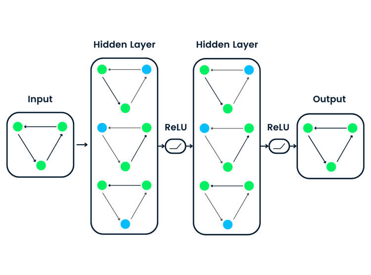
The main difference between KANs and traditional Multi-Layer Perceptrons (MLPs) lies in how learning occurs.

In MLPs, neurons are activated using fixed functions like ReLU or sigmoid, and these activations are passed through linear weight matrices. By contrast, KANs place learnable activation functions on the edges (connections) between neurons rather than at the neurons themselves. In the original implementation, these functions are parameterized as B-splines, though the authors mention that other types of functions, such as Chebyshev polynomials, can also be used depending on the problem.

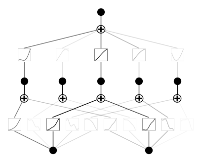
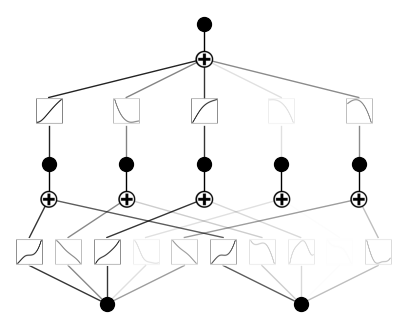
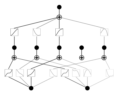
Both shallow and deep KANs break down complex functions into a series of simpler, univariate ones. The figure below highlights this difference in architecture: MLPs use fixed activations within the neurons, while KANs implement learnable functions along the edges and sum them on nodes. This architectural shift allows KANs to adapt dynamically to the data, potentially achieving greater accuracy with fewer parameters than MLPs. Furthermore, after the training, the model can be made smaller when not all the edges are used for approximation.

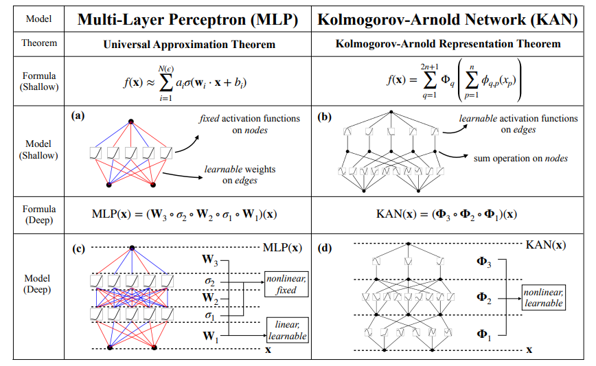
Source: Liu et al., 2024

Moreover, after training, KANs allow us to extract the learned univariate functions, making it possible to reconstruct the resulting multivariable function. This feature is particularly useful when interpretability is crucial. We will showcase this process in the examples section later on.

pip install git+https://github.com/KindXiaoming/pykan.git

Usage

After installing pykan, we can start importing the necessary modules and defining a simple KAN:

from kan import *
model = KAN(width=[2,5,1])

Here, we specify the dimensions of the model in the width parameter. In this particular case, we are making a model with 2 inputs, 1 output, and a layer of 5 hidden neurons.Now, let’s create a dataset for our experiment. I will use a random 2-variable polynomial I just came up with on the fly:

from kan.utils import create_dataset
f = lambda x: 3*x[:,[0]]**3+2*x[:,[0]]+4 + 2 * x[:,[0]] * x[:,[1]] ** 2 + 3 * x[:,[1]] ** 3
dataset = create_dataset(f, n_var=2)

Here, I use a lambda function to define a polynomial. The library seems to use the numpy library under the hood—hence the syntax. Now, we can load the dataset into a model and visualize it:

model(dataset['train_input']);
model.plot()

Here is what the output looks like:

Training

In order to run training, we need to use the .fit() method:

model.fit(dataset, steps=1000);

After the training, this is what our KAN looks like:

Now, let's prune and plot the model again:

model = model.prune()
model.plot()

Here is what the model looks like now. As you can see, we pruned one activation function:

This makes sense, because our polynomial does not use five different combinations of powers of input variables.

Use Cases of KANs

Kolmogorov-Arnold Networks (KANs) have shown promise across various fields due to their ability to model complex, non-linear relationships with fewer parameters than traditional neural networks. Here are some key use cases:

• Scientific modeling and data fitting: KANs are particularly effective for scientific problems that require accurate modeling of complex functions. Since KANs approximate multivariable functions by learning simpler univariate ones, they can efficiently capture intricate patterns in scientific data. For tasks like curve fitting, KANs often outperform traditional MLPs due to their flexible architecture.
• Solving partial differential equations (PDEs): KANs have demonstrated strong potential in solving PDEs, which are commonly used in physics and engineering to model processes like heat transfer and fluid dynamics. Their capacity to handle high-dimensional, non-linear problems makes them particularly useful in this domain, surpassing MLPs in accuracy and interpretability.
• Symbolic regression: KANs excel in symbolic regression, where the goal is to uncover mathematical expressions that best describe a dataset. Their ability to learn compositional structures makes them an ideal tool for rediscovering physical and mathematical laws directly from data.

Advantages and Disadvantages of KANs

Let's explore some of the ways KANs improve upon the limitations of conventional neural networks:

• Interpretability: Unlike traditional deep learning models, KANs provide a more interpretable structure. The learnable functions can be visualized and analyzed, offering insights into the model's decision-making process. This characteristic is particularly valuable in scientific fields, where understanding the model's workings is just as crucial as achieving high accuracy.
• Flexibility: KANs are not limited to a single type of activation function. While they often use B-splines, other basis functions, such as Chebyshev polynomials, can be employed based on the specific task. This flexibility makes the architecture versatile and adaptable to a range of applications.

KANs present a promising new approach to deep learning, but like any technology, they come with their own weaknesses:

• Computational complexity: One of the challenges with KANs is their computational intensity during the training phase. Since KANs use learnable activation functions on the edges, the complexity of evaluating these functions can significantly slow down the training process compared to traditional MLPs. This complexity is further amplified in tasks that require deep KAN architectures or highly detailed basis functions.
• Need for expertise: Implementing and tuning KANs can be more complex than working with traditional MLPs. Selecting the appropriate basis functions (e.g., B-splines, Chebyshev polynomials) and configuring the model for a specific task require a deeper mathematical understanding and more human/model interaction. This can make KANs less accessible to practitioners without specialized knowledge.

Human-KAN Interaction

A unique aspect of Kolmogorov-Arnold Networks (KANs) is their ability to facilitate meaningful interaction between the model and human intuition. The original paper describes how researchers can engage with the model's learning in ways not possible with traditional neural networks.

After training a KAN on a specific problem, researchers can extract the learned univariate functions that the model uses to approximate the complex multivariable function. By studying these learned functions, researchers gain insights into the underlying relationships in the data.

Furthermore, the insights gained from this interaction enable iterative refinement. Researchers can tweak the KAN's architecture, modify the types of basis functions (e.g., switching from B-splines to Chebyshev polynomials), or adjust the training process based on the extracted functions. This human-in-the-loop approach allows for a tailored modeling process, making KANs adaptable to different scientific or mathematical problems.

In this way, KANs facilitate a two-way interaction: they learn from data to form complex functions, and humans can guide and interpret this learning to refine the model or even uncover new knowledge. This interplay is what makes KANs stand out, transforming machine learning into a more collaborative and exploratory endeavor.

Conclusion

Overall, Kolmogorov-Arnold Networks (KANs) represent an exciting and promising advancement in neural network architecture. Their unique design offers a flexible and interpretable alternative to MLPs, with the potential to outperform traditional models in various tasks.

As the community continues to explore KANs through open-source collaborations and diverse applications, these networks and their extensions could evolve into powerful, state-of-the-art tools.