A Comprehensive Introduction to Graph Neural Networks (GNNs)

What is a Graph?

A Graph is the type of data structure that contains nodes and edges. A node can be a person, place, or thing, and the edges define the relationship between nodes. The edges can be directed and undirected based on directional dependencies. 

In the example below, the blue circles are nodes, and the arrows are edges. The direction of edges defines dependencies between two nodes. 

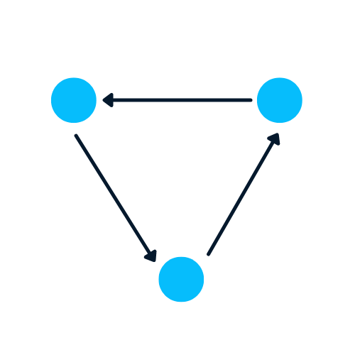
Image by Author 

Let’s learn about the complex Graph dataset: Jazz Musicians Network. It contains 198 nodes and 2742 edges. In the community graph plot below, different colors of nodes represent various communities of Jazz musicians and the edges connecting them. There is a web of collaboration where a single musician has relationships within and outside the community. 

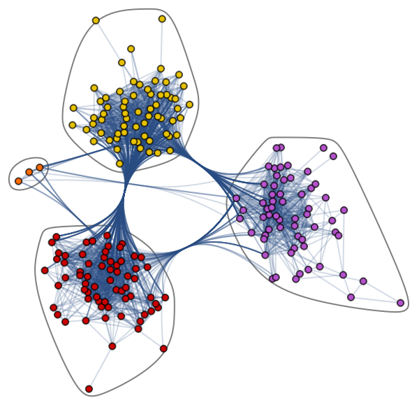
 Community Graph Plot by Jazz Musicians Network

Graphs are excellent in dealing with complex problems with relationships and interactions. They are used in pattern recognition, social networks analysis, recommendation systems, and semantic analysis. Creating graph-based solutions is a whole new field that offers rich insights into complex and interlinked datasets.

Graphs with NetworkX

In this section, we will learn to create a graph using NetworkX. 

The code below is influenced by Daniel Holmberg's blog on Graph Neural Networks in Python.

1. Create networkx’s DiGraph object “H”
2. Add nodes that contain different labels, colors, and size
3. Add edges to create a relationship between two nodes. For example, “(0,1)” means that 0 has a directional dependency on 1. We will create bidirectional relationships by adding “(1,0)”
4. Extract colors and sizes in the form of lists
5. Plot the graph using networkx’s draw function

import networkx as nx
H = nx.DiGraph()

#adding nodes
H.add_nodes_from([
  (0, {"color": "blue", "size": 250}),

  (1, {"color": "yellow", "size": 400}),

  (2, {"color": "orange", "size": 150}),

  (3, {"color": "red", "size": 600})


])

#adding edges
H.add_edges_from([
  (0, 1),

  (1, 2),

  (1, 0),

  (1, 3),

  (2, 3),

  (3,0)


])

node_colors = nx.get_node_attributes(H, "color").values()
colors = list(node_colors)
node_sizes = nx.get_node_attributes(H, "size").values()
sizes = list(node_sizes)

#Plotting Graph
nx.draw(H, with_labels=True, node_color=colors, node_size=sizes)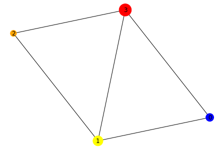

In the next step, we will convert the data structure from directional to an undirectional graph using the to_undirected() function. 

#converting to undirected graph
G = H.to_undirected()
nx.draw(G, with_labels=True, node_color=colors, node_size=sizes)

Why is it Hard to Analyze a Graph?

Graph-based data structures have drawbacks, and data scientists must understand them before developing graph-based solutions.

1. A graph exists in non-euclidean space. It does not exist in 2D or 3D space, which makes it harder to interpret the data. To visualize the structure in 2D space, you must use various dimensionality reduction tools.
2. Graphs are dynamic; they do not have a fixed form. There can be two visually different graphs, but they might have similar adjacency matrix representations. It makes it difficult for us to analyze data using traditional statistical tools. 
3. Large size and dimensionality will increase the graph's complexity for human interpretations. The dense structure with multiple nodes and thousands of edges is harder to understand and extract insights. 

What is a Graph Neural Network (GNN)?

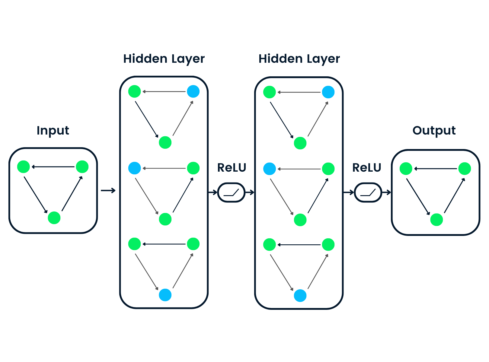
Graph Neural Networks are special types of neural networks capable of working with a graph data structure. They are highly influenced by Convolutional Neural Networks (CNNs) and graph embedding. GNNs are used in predicting nodes, edges, and graph-based tasks. 

• CNNs are used for image classification. Similarly, GNNs are applied to graph structure (grid of pixels) to predict a class. 
• Recurrence Neural Networks are used in text classification. Similarly, GNNs are applied to graph structures where every word is a node in a sentence.  

GNNs were introduced when Convolutional Neural Networks failed to achieve optimal results due to the arbitrary size of the graph and complex structure. 

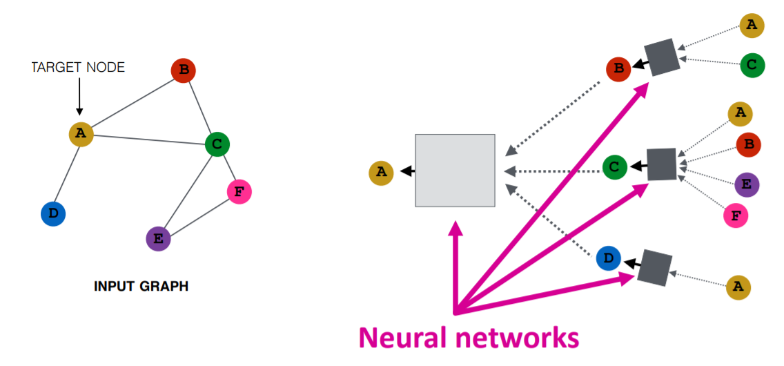
Image by Purvanshi Mehta

The input graph is passed through a series of neural networks. The input graph structure is converted into graph embedding, allowing us to maintain information on nodes, edges, and global context. 

Then the feature vector of nodes A and C is passed through the neural network layer. It aggregates these features and passes them to the next layer - neptune.ai.

Read our Deep Learning tutorial or take our Introduction to Deep Learning course to learn more about deep learning algorithms and applications. 

Types of Graph Neural Networks

There are several types of neural networks, and most of them have some variation of Convolutional Neural Networks. In this section, we will be learning about the most popular GNNs. 

• Graph Convolutional Networks (GCNs) are similar to traditional CNNs. It learns features by inspecting neighboring nodes. GNNs aggregate node vectors, pass the result to the dense layer, and apply non-linearity using the activation function. In short, it consists of Graph convolution, linear layer, and non-learner activation function. There are two major types of GCNs: Spatial Convolutional Networks and Spectral Convolutional Networks.
• Graph Auto-Encoder Networks learn graph representation using an encoder and attempt to reconstruct input graphs using a decoder. The encoder and decoders are joined by a bottleneck layer. They are commonly used in link prediction as Auto-Encoders are good at dealing with class balance. 
• Recurrent Graph Neural Networks(RGNNs) learn the best diffusion pattern, and they can handle multi-relational graphs where a single node has multiple relations. This type of graph neural network uses regularizers to boost smoothness and eliminate over-parameterization. RGNNs use less computation power to produce better results. They are used in generating text, machine translation, speech recognition, generating image descriptions, video tagging, and text summarization.
• Gated Graph Neural Networks (GGNNs) are better than the RGNNs in performing tasks with long-term dependencies. Gated Graph Neural Networks improve Recurrent Graph Neural Networks by adding a node, edge, and time gates on long-term dependencies. Similar to Gated Recurrent Units (GRUs), the gates are used to remember and forget information in different states. 

If you are interested in learning more about Recurrent Neural Networks (RNNs), check out DataCamp’s course. It will introduce you to various RNNs model architectures, Keras frameworks, and RNN applications. 

Types of Graph Neural Networks Tasks

Below, we’ve outlined some of the types of GNN tasks with examples:

• Graph Classification: we use this to classify graphs into various categories. Its applications are social network analysis and text classification. 
• Node Classification: this task uses neighboring node labels to predict missing node labels in a graph. 
• Link Prediction: predicts the link between a pair of nodes in a graph with an incomplete adjacency matrix. It is commonly used for social networks. 
• Community Detection: divides nodes into various clusters based on edge structure. It learns from edge weights, and distance and graph objects similarly. 
• Graph Embedding: maps graphs into vectors, preserving the relevant information on nodes, edges, and structure.
• Graph Generation: learns from sample graph distribution to generate a new but similar graph structure. 

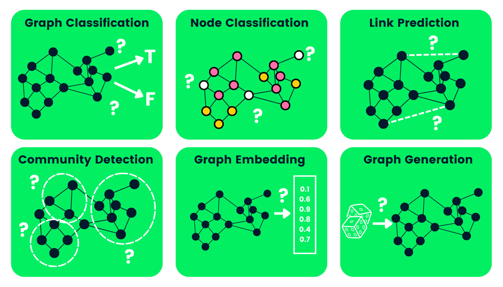
Image by Author

Disadvantages of Graph Neural Networks

There are a few drawbacks to using GNNs. Understanding them will help us determine when to use GNNa and how to optimize the performance of our machine learning models. 

1. Most neural networks can go deep to obtain better performance, whereas GNNs are shallow networks mostly with three layers. It limits us from achieving state-of-the-art performance on large datasets.
2. The graph structures are constantly changing, making it harder to train a model on it. 
3. Deploying the model to production faces scalability issues as these networks are computationally expensive. If you have a large and complex graph structure, it will be hard for you to scale the GNNs in production. 

What is a Graph Convolutional Network (GCN)?

The majority of GNNs are Graph Convolutional Networks, and it is important to learn about them before jumping into a node classification tutorial.  

The convolution in GCN is the same as a convolution in convolutional neural networks. It multiplies neurons with weights (filters) to learn from data features. 

It acts as sliding windows on whole images to learn features from neighboring cells. The filter uses weight sharing to learn various facial features in image recognition systems - Towards Data Science. 

Now transfer the same functionality to Graph Convolutional networks where a model learns the features from neighboring nodes. The major difference between GCN and CNN is that it is developed to work on non-euclidean data structures where the order of nodes and edges can vary. 

CNN vs GCN | Image Source

Learn more about basic CNNs by following Convolutional Neural Networks (CNN) with the TensorFlow tutorial. 

There are two types of GCNs: 

• Spatial Graph Convolutional Networks use spatial features to learn from graphs that are located in spatial space.  
• Spectral Graph Convolutional Networks use Eigen-decomposition of graph Laplacian matrix for information propagation along nodes. These networks were inspired by wave propagation in signals and systems. 

How do GNNs Work? Building a Graph Neural Network with Pytorch

We will build and train Spectral Graph Convolution for a node classification model. The code source is available on Workspace for you to experience and run your first graph-based machine learning model. 

The coding examples are influenced by Pytorch geometric documentation. 

Getting Started

We will install the Pytorch package as pytorch_geometric is built upon it. 

!pip install -q torch

Then we will use the torch version to install torch-scatter and torch-sparse. After that, we will install pytorch_geometric’s latest release from GitHub. 

%%capture
import os
import torch
os.environ['TORCH'] = torch.__version__
os.environ['PYTHONWARNINGS'] = "ignore"
!pip install torch-scatter -f https://data.pyg.org/whl/torch-${TORCH}.html
!pip install torch-sparse -f https://data.pyg.org/whl/torch-${TORCH}.html
!pip install git+https://github.com/pyg-team/pytorch_geometric.git

Planetoid Cora Dataset

Planetoid is a citation network dataset from Cora, CiteSeer, and PubMed. The nodes are documents with 1433-dimensional bag-of-words feature vectors, and the edges are citation links between research papers. There are 7 classes, and we will train the model to predict missing labels. 

We will ingest the Planetoid Cora dataset, and row normalize the bag of words input features. After that, we will analyze the dataset and the first graph object. 

from torch_geometric.datasets import Planetoid
from torch_geometric.transforms import NormalizeFeatures

dataset = Planetoid(root='data/Planetoid', name='Cora', transform=NormalizeFeatures())

print(f'Dataset: {dataset}:')
print('======================')
print(f'Number of graphs: {len(dataset)}')
print(f'Number of features: {dataset.num_features}')
print(f'Number of classes: {dataset.num_classes}')

data = dataset[0]  # Get the first graph object.
print(data)

The Cora dataset has 2708 nodes, 10,556 edges, 1433 features, and 7 classes. The first object has 2708 train, validation, and test masks. We will use these masks to train and evaluate the model. 

Dataset: Cora():
======================
Number of graphs: 1
Number of features: 1433
Number of classes: 7
Data(x=[2708, 1433], edge_index=[2, 10556], y=[2708], train_mask=[2708], val_mask=[2708], test_mask=[2708])

Node Classification with GNN

We will create a GCN model structure that contains two GCNConv layers relu activation and a dropout rate of 0.5. The model consists of 16 hidden channels.  

GCN layer:

The W(ℓ+1) is a tranable weight matrix in above equation and Cw,v donestes to a fixed normalization coefficient for each edge.

from torch_geometric.nn import GCNConv
import torch.nn.functional as F

class GCN(torch.nn.Module):
    def __init__(self, hidden_channels):
        super().__init__()
        torch.manual_seed(1234567)
        self.conv1 = GCNConv(dataset.num_features, hidden_channels)
        self.conv2 = GCNConv(hidden_channels, dataset.num_classes)

    def forward(self, x, edge_index):
        x = self.conv1(x, edge_index)
        x = x.relu()
        x = F.dropout(x, p=0.5, training=self.training)
        x = self.conv2(x, edge_index)
        return x

model = GCN(hidden_channels=16)
print(model)

>>> GCN(
    (conv1): GCNConv(1433, 16)
    (conv2): GCNConv(16, 7)
  )

Visualizing Untrained GCN network

Let’s visualize node embeddings of untrained GCN networks using sklearn.manifold.TSNE and matplotlib.pyplot. It will plot a 7 dimension node embedding a 2D scatter plot.  

%matplotlib inline
import matplotlib.pyplot as plt
from sklearn.manifold import TSNE

def visualize(h, color):
    z = TSNE(n_components=2).fit_transform(h.detach().cpu().numpy())

    plt.figure(figsize=(10,10))
    plt.xticks([])
    plt.yticks([])

    plt.scatter(z[:, 0], z[:, 1], s=70, c=color, cmap="Set2")
    plt.show()

We will evaluate the model then add training data to the untrained model to visualize various nodes and categories. 

model.eval()

out = model(data.x, data.edge_index)
visualize(out, color=data.y)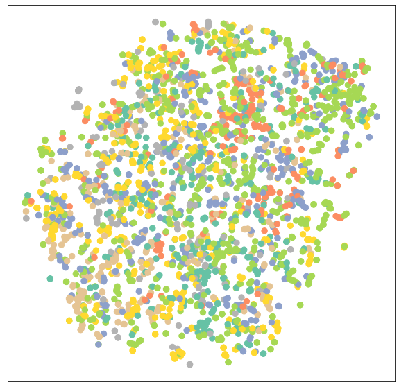

Training GNN

We will train our model on 100 Epochs using Adam optimization and the Cross-Entropy Loss function. 

In the train function, we have:

1. Clear the gradient
2. Performed a single forward pass
3. Compute loss using training nodes
4. Calculate gradient, and update the parameters

In the test function, we have:

1. Predicted node class
2. Extracted class label with the highest probability
3. Checked how many values have been predicted correctly
4. Creating accuracy ratio using a sum of correct predictions divided by a total number of nodes. 

model = GCN(hidden_channels=16)
optimizer = torch.optim.Adam(model.parameters(), lr=0.01, weight_decay=5e-4)
criterion = torch.nn.CrossEntropyLoss()

def train():
      model.train()
      optimizer.zero_grad()
      out = model(data.x, data.edge_index)
      loss = criterion(out[data.train_mask], data.y[data.train_mask])
      loss.backward()
      optimizer.step()
      return loss

def test():
      model.eval()
      out = model(data.x, data.edge_index)
      pred = out.argmax(dim=1)
      test_correct = pred[data.test_mask] == data.y[data.test_mask]
      test_acc = int(test_correct.sum()) / int(data.test_mask.sum())
      return test_acc


for epoch in range(1, 101):
    loss = train()
    print(f'Epoch: {epoch:03d}, Loss: {loss:.4f}')
GAT(
  (conv1): GATConv(1433, 8, heads=8)
  (conv2): GATConv(64, 7, heads=8)
)

.. .. .. ..
.. .. .. ..
Epoch: 098, Loss: 0.5989
Epoch: 099, Loss: 0.6021
Epoch: 100, Loss: 0.5799

Model Evaluation

We will now evaluate the model on an unseen dataset using the test function, and as you can see, we got pretty good results on 81.5% accuracy.  

test_acc = test()
print(f'Test Accuracy: {test_acc:.4f}')


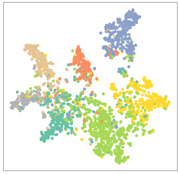
>>> Test Accuracy: 0.8150

We will now visualize the output embedding of a trained model to verify the results.

model.eval()
out = model(data.x, data.edge_index)
visualize(out, color=data.y)

As we can see, the trained model has produced better clustering of nodes for the same category.

Training GATConv Model

In the second, we will replace GCNConv with GATConv layers. The Graph Attention Networks uses masked self-attentional layers to address the drawbacks of GCNConv and achieve state-of-the-art results. 

You can also try other GNN layers and play around with optimizations, dropouts, and a number of hidden channels to achieve better performance. 

In the code below, we have just replaced GCNConv with GATConv with 8 attention heads in the first layer and 1 in the second layer. 

We will also set:

• dropout rate to 0.6
• hidden channels to 8
• learning rate 0.005

We have modified the test function to find the accuracy of a specific mask (valid, test). It will help us print out validation and test scores during model training. We are also storing validation and test results to a plot line chart later. 

from torch_geometric.nn import GATConv

class GAT(torch.nn.Module):
    def __init__(self, hidden_channels, heads):
        super().__init__()
        torch.manual_seed(1234567)
        self.conv1 = GATConv(dataset.num_features, hidden_channels,heads)
        self.conv2 = GATConv(heads*hidden_channels, dataset.num_classes,heads)

    def forward(self, x, edge_index):
        x = F.dropout(x, p=0.6, training=self.training)
        x = self.conv1(x, edge_index)
        x = F.elu(x)
        x = F.dropout(x, p=0.6, training=self.training)
        x = self.conv2(x, edge_index)
        return x

model = GAT(hidden_channels=8, heads=8)
print(model)

optimizer = torch.optim.Adam(model.parameters(), lr=0.005, weight_decay=5e-4)
criterion = torch.nn.CrossEntropyLoss()

def train():
      model.train()
      optimizer.zero_grad()
      out = model(data.x, data.edge_index)
      loss = criterion(out[data.train_mask], data.y[data.train_mask])
      loss.backward()
      optimizer.step()
      return loss

def test(mask):
      model.eval()
      out = model(data.x, data.edge_index)
      pred = out.argmax(dim=1)
      correct = pred[mask] == data.y[mask]
      acc = int(correct.sum()) / int(mask.sum())
      return acc

val_acc_all = []
test_acc_all = []

for epoch in range(1, 101):
    loss = train()
    val_acc = test(data.val_mask)
    test_acc = test(data.test_mask)
    val_acc_all.append(val_acc)
    test_acc_all.append(test_acc)
    print(f'Epoch: {epoch:03d}, Loss: {loss:.4f}, Val: {val_acc:.4f}, Test: {test_acc:.4f}')

.. .. .. ..
.. .. .. ..
Epoch: 098, Loss: 1.1283, Val: 0.7960, Test: 0.8030

Epoch: 099, Loss: 1.1352, Val: 0.7940, Test: 0.8050

Epoch: 100, Loss: 1.1053, Val: 0.7960, Test: 0.8040

As we can observe, our model didn’t perform better than GCNConv. It requires hyperparameter optimization or more Epochs to achieve state-of-the-art results. 

Model Evaluation

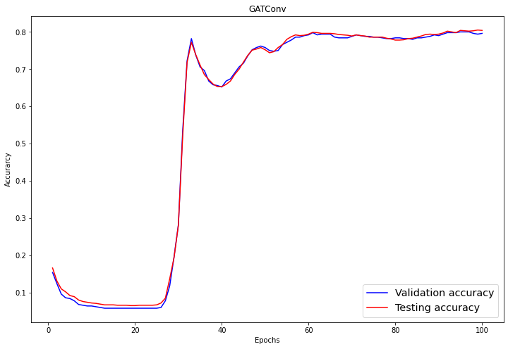
In the evaluation part, we visualize validation and testing scores using matplotlib.pyplot’s line plot.  

import numpy as np

plt.figure(figsize=(12,8))
plt.plot(np.arange(1, len(val_acc_all) + 1), val_acc_all, label='Validation accuracy', c='blue')
plt.plot(np.arange(1, len(test_acc_all) + 1), test_acc_all, label='Testing accuracy', c='red')
plt.xlabel('Epochs')
plt.ylabel('Accurarcy')
plt.title('GATConv')
plt.legend(loc='lower right', fontsize='x-large')
plt.savefig('gat_loss.png')
plt.show()

Ater 60 Epochs, the validation, and testing accuracy has achieved a stable value of 0.8+/-0.02. 

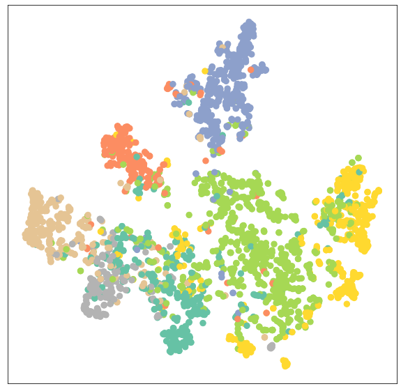
Again, let’s visualize the node clustering of the GATConv model.

model.eval()

out = model(data.x, data.edge_index)
visualize(out, color=data.y)

As we can see, the GATConv layer has produced the same results in clustering on the same category of nodes. 

We can reduce overfitting by adding a second validation dataset and improve model performance by experimenting with various GCN layers from pytoch_geometric. 

The source code of the tutorial is available on DataCamp Workspace. You just need to click on the Copy & Edit button and run the Jupyter Notebook. 

Add Deep Learning skill to your Résumé by taking Deep Learning in Python skill track. It will introduce you to deep learning algorithms, Keras, Pytorch, and the Tensorflow framework.