How to Merge Two Columns in Excel: Simple Formulas and More

Merging columns saves time and avoids mistakes. It’s a simple trick that makes managing data less frustrating. In this guide, I’ll show you the different steps I use to merge Excel columns so you can try them out for yourself, too.

After this article, enroll in our Introduction to Excel course so you can be ready to handle the next challenge that comes along.

The Quick Answer

To merge two columns in Excel, use the ampersand to concatenate text from different cells and add a space between the text strings if needed.

=A2 & " " & B2

Here, the & combines the text, and the " " adds a space between the first and last names. When I hit Enter, both columns are combined into one.

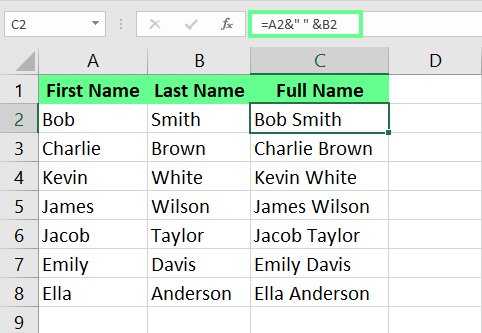
Combine columns using &. Image by Author.

All the Ways to Merge Two Columns in Excel

Now, let's go through all the methods.

Using the CONCAT() function

The CONCAT() function is an option. The CONCAT() function explicitly concatenates the arguments you pass to it. 

For example, when I enter the following formula in cell C2, CONCAT() combines data from both columns: 

=CONCAT(A2, " ", B2)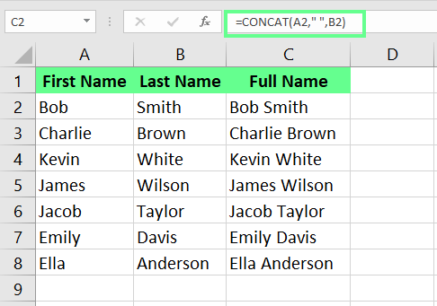

Combine columns with the CONCAT() function. Image by Author.

You might be wondering how CONCAT() is different than the ampersand. Essentially, there's no difference and they achieve the same result.

Note: If you’re using an older version of Excel (older than 2016), you’ll have the CONCATENATE() function instead of CONCAT(). But it works the same way, so don’t worry.

Using the TEXTJOIN() function

The TEXTJOIN() function merges text from multiple columns that contain a specific delimiter. For example, I select cell C2 and enter the following formula: 

=TEXTJOIN(" ", TRUE, A2, B2)

In this formula, I’ve used the space " " delimiter to separate the text, and the TRUE argument ensures that any blank cells are ignored. Once I press Enter, the names are merged into one cell with a space between them.

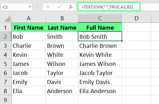
Combine cells using the TEXTJOIN() function. Image by Author.

Using Flash Fill

Sometimes, I use the built-in Flash Fill option. Flash Fill is convenient because it automatically detects patterns and applies them to the rest of the column. 

Here’s how it works: In cell C2, I manually type the full name. Then, in cell C3, as I start typing the next name, Excel suggests the rest of the cells in the same format. I press Enter, and the entire column is filled with the combined names. Just make sure that your first entry looks exactly how you want the rest to follow, otherwise a mistake will be applied throughout.

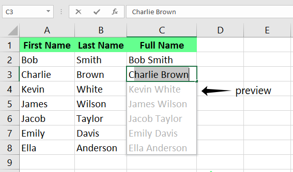
Combine columns using Flash Fill. Image by Author.

If you don't see the preview, it may be because the flash fill is not turned on. To turn it on:

• Go to File > Options > Advanced > Editing options
• Check the Automatically Flash Fill box.

You can also manually run it by going to the Data tab and clicking on the Flash Fill option, or you could use a shortcut key, Ctrl + E.

Using Power Query

If you work with large datasets with so many columns, I’d suggest using Power Query to merge columns. It handles big data without slowing things down, and the best part is that it updates automatically if the source data changes. It also keeps original data safe, so you don’t have to worry about mistakes.  

Click anywhere on the dataset. Then, go to the Data tab and click on From Table/Range. A Create Table dialog box will appear. Check the My table has headers box and click OK.

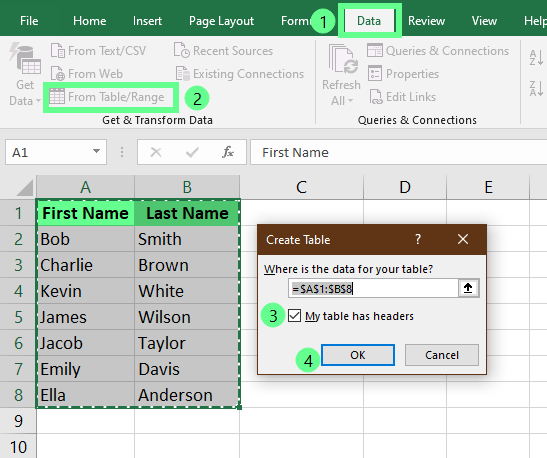
Open Power Query Editor. Image by Author.

A Power Query Editor window will appear. To select both columns, hold Ctrl and click on the columns. Then, choose Add Column from the ribbon and click Merge Columns.

In this example, I select a Space separator in the dialog box from the drop-down menu, name my column Full Name, and click OK.

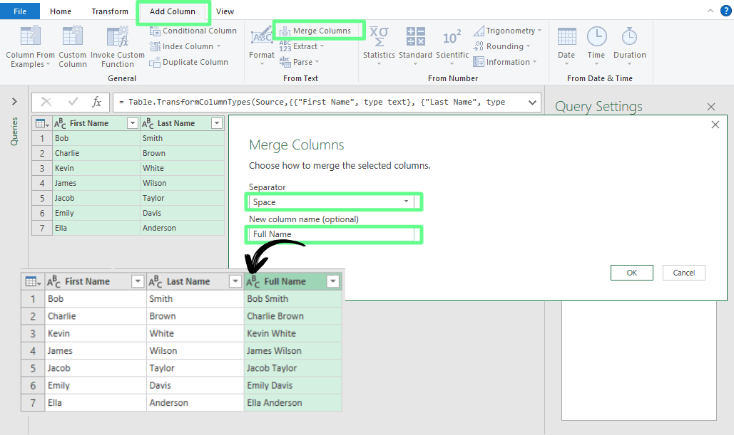
Merge columns using Power Query. Image by Author.

Once the new merged column is added, go to the Home tab and click Close & Load to export it to your worksheet.

Using Notepad as an intermediary

This may surprise you, but Notepad can also merge data. However, it only helps when the columns are next to each other and have the same separator.

I'll show you how: Click on cell A2, and select the adjacent column B2, I press Shift + Right Arrow, then Ctrl + Shift + Down Arrow to select both the columns’ data. 

Next, I copy the data and paste it on the notepad. Then, I press the Tab key in Notepad. Now, I open the Replace dialog box by pressing Ctrl+H and I paste the Tab character in the Find What field. I enter the separator (Space) in the Replace with field. After this, I copy all the data and paste it into Excel.

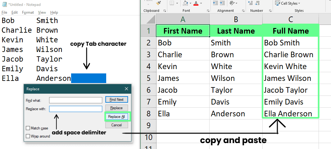
Merge cells using Notepad. Image by Author.

You might be wondering why I would consider Notepad, as it seems like more work. But, because Notepad is a plain text editor that automatically removes any hidden characters, by copying data from Excel to Notepad, I know that only the raw text remains. I'm bringing this up because, in some cases, I was working with data that had complex formatting, or non-printable or non-binary characters, or some other kind of artifacts, and I had problems, in which case, I have to say, Notepad helped.

Using Add-ins

Add-ins make work so much easier. I rely on the Merge Cells add-in to quickly combine data from different cells using separators like spaces or commas. 

You can use the Ultimate Suite for this. Once it's downloaded, open the Excel worksheet, and it will appear in the ribbon. Then, select the cells you want to merge and go to Ablebits Data > Merge Cells > Merge Columns into One.

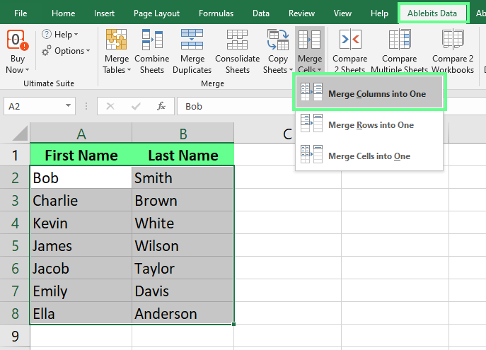
Select two columns to merge into one. Image by Author.

A Merge Cells dialog box will appear. In the How to merge option, select Columns into one and choose any delimiter (in my case, it’s a space) in the Combine with field. In my example, I set the Place the results to field to the left column because that’s where I want the merged data to show up. I check the box for Clear the contents of the selected cells to keep things clean and click Merge.

The advantage here is that I can merge the columns without using any formulas.

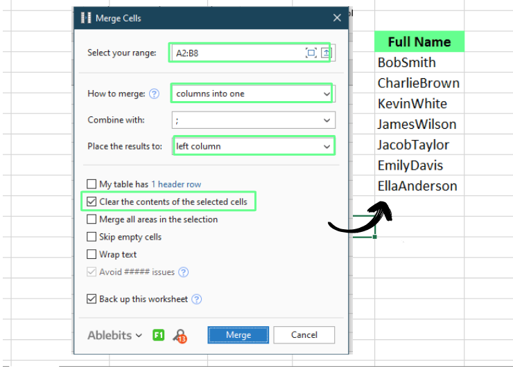
Merge cells using Add-ins. Image by Author.

Using the Merge & Center tool

This one is a little different because it makes the cell longer than the others, but still, it has its uses.

Excel has a built-in tool called Merge & Center that combines multiple cells into one. However, it only keeps the data from the top-left cell, and anything in the other cells gets deleted. I mostly use it to create a single header or title across multiple columns.

For example, if I want to create a header that reads Students on top of columns A, B and C, I type Students in cell A2, then select the cells from A2 to C2. Next, I click Merge & Center in the Home tab. This way, these cells merge into one, and the text is perfectly centered, giving a clean and organized heading look.

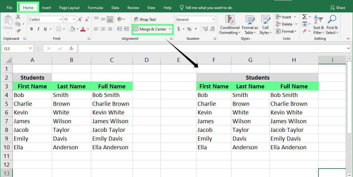
Merge cells using the Merge and Center tool. Image by Author.

Using the ampersand (&) symbol

Finally, I will review the method I used at the top of the article. Here, I have a dataset of names, and I want to combine them. I type the following formula in cell C2:

=A2 & " " & B2

Combine columns using ampersand. Image by Author.

A quick overview of all the methods

Now that we have covered all the functions, let’s quickly compare them to see where each stands out and what it lacks. 

Tips and Best Practices 

Here are a few tips for merging cells in Excel that have made my work much easier, and I’m sure they’ll help you, too:

• Preserve formatting: Excel formulas don’t maintain the cell formatting. So, to make sure your data looks consistent, use tools like Merge Cells or an Excel Add-in.

• Handle large datasets: When I work with large datasets, I use Power Query or Excel Add-ins because they make the process smoother and handle vast amounts of data efficiently.

• Use the correct delimiters: Always choose the right delimiter when you merge data. Whether it’s a space, a comma, or something else.
• Convert formulas to values: When I’m done merging, I convert formulas into static values. Just copy the cells and use the Paste Special > Values option. This will lock in the results and remove the formulas.

Conclusion 

I’ve covered everything about merging columns in Excel and how it can help you avoid errors. If you want to learn more about Excel and take your skills to the next level, check out our Data Preparation in Excel course — it’s great for mastering how to organize and clean data efficiently. If you want to focus on creating charts and graphs, we have Data Visualization in Excel - another great options.