Course
Introduction to Regression in R
4 hr
77.1K
Conducting thorough research is complex and requires careful planning, including how participants are assigned to treatment groups that include the treatment (or in other words, the intervention) vis-a-vis control groups where they don’t.
One such approach is randomly assigning participants to either group to minimize bias. This random assignment helps attribute the differences in outcomes to the treatment, rather than to other variables. However, random assignments are not always possible due to ethical, practical, or logistical limitations. In such cases, the researchers resort to alternatives, such as observational studies as they rely on simply observing what naturally occurs in the real world. While valuable, these research designs can lead to selection bias, influencing the outcomes of the study.
To address the issue of selection bias, researchers often use propensity scores—and that’s the focus of this post. When you are finished, I hope you take our courses to build a strong foundation in causal thinking. Start with Foundations of Inference in Python to understand core principles like sampling distributions. Then, move on to Intermediate Regression in Python for hands-on experience with modeling (this is an essential skill for estimating causal effects). Inference for Linear Regression in R is another great option. Now, let's get started!
We understand that there are situations where random assignment is not an option. To add to that, we must address selection bias too. This is where a method called propensity score is used to balance groups in observational studies. A propensity score is the probability that a participant would receive a particular treatment based on their observed characteristics.
This method was developed by Rosenbaum and Rubin in the 1980s and has been widely used in healthcare, social sciences, and economics. Here’s how it works:
Before we proceed further, let’s understand what confounding means. Confounding occurs when an outside variable, known as a confounding variable or confounder, influences both the independent variable (treatment) and the dependent variable (outcome), potentially leading to incorrect conclusions about the relationship between them.
For example, physical exercise is a confounder for a study examining whether drinking coffee (independent variable) is associated with higher productivity (dependent variable). That’s because people who exercise more may also drink more coffee and have higher productivity, which makes it difficult to tell if coffee alone influences productivity or if exercise is partly responsible.
In this case, exercise, the confounding factor, could mislead researchers by falsely suggesting a stronger relationship between coffee and productivity than might exist.
The four primary methods for applying propensity scores in observational studies are matching, stratification, inverse probability weighting, and covariate adjustment. Let’s discuss each of them in detail.
Propensity score matching pairs the participants from the treatment group with participants from the control group who have similar propensity scores. This pairing process takes into account that the groups are as similar as possible, thereby reducing the possibility of bias. In other words, the individuals with comparable probabilities of receiving the treatment are paired to create a balanced sample.
Matching is ideal when the goal is to create directly comparable groups and reduce differences in characteristics as much as possible. Having a moderate to large sample size is preferable, as it facilitates finding good matches.
In a study assessing the impact of remote work on employee productivity, researchers could match employees working remotely (treatment) with similar employees working on-site (control) based on variables such as job role, years of experience, and previous performance metrics. This would allow researchers to compare productivity outcomes while reducing the impact of background differences.
Stratification is the process of dividing participants into distinct groups, also called strata, based on their propensity scores. Often, these groups are divided into quintiles, i.e., five equal parts. Each stratum contains participants with similar propensity scores, and outcomes within each stratum are compared between treatment and control groups.
This method is effective when the sample size is large enough to create several meaningful strata, as fewer participants per stratum might not lead to effective comparisons.
To assess the effectiveness of a new medication as part of a healthcare study, patients can be stratified into quintiles based on propensity scores calculated from demographics and baseline health conditions. Each stratum can include patients with similar characteristics, which leads to more accurate treatment effect comparisons within each group.
IPW assigns weights based on propensity scores to give more "importance" to certain observations when estimating treatment effects. Participants with a lower likelihood of being in their respective groups are given more weight to balance differences in group characteristics.
Considering that it proportionally leverages data from both groups, IPW is preferred when researchers need to generalize findings to the entire sample population.
In a public health study evaluating a community intervention, IPW could be applied to account for demographic and socio-economic differences between communities that received the intervention and those that did not. This allows for generalizable findings without creating matched pairs. Here are steps:
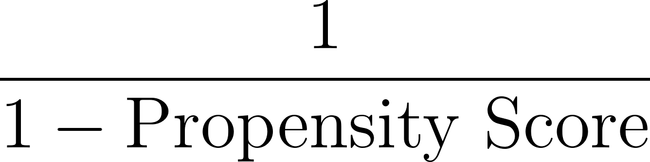
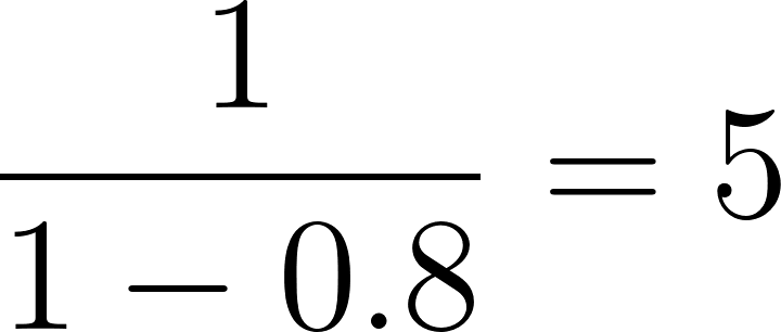
Next, we calculate weights based on the inverse of the propensity score, as shown below:

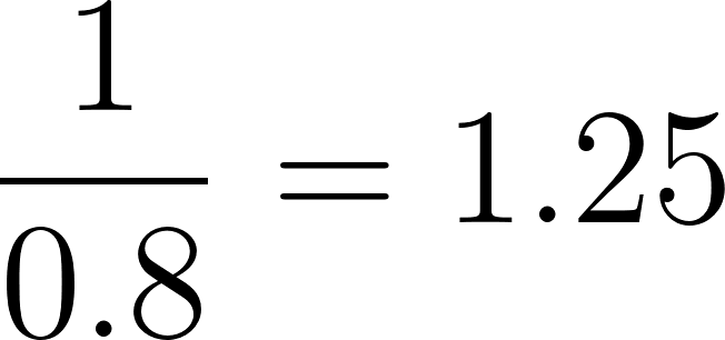
In our example, for the individual with a propensity score of 0.8:
Now, apply these weights to each individual in the study to create a "pseudo-population" where each individual’s influence on the analysis is adjusted by their weight. This pseudo-population balances the baseline characteristics across the treatment and control groups. In the resulting pseudo-population, the likelihood of an individual being in the treatment or control group is independent of their baseline characteristics, thus reducing confounding.
As a note, IPTW can be used to address a large number of confounding variables. It can also be applied to longitudinal studies to account for time-dependent confounding.
Some other important considerations when using IPTW include:
In covariate adjustment, we use the propensity scores as an additional covariate variable in a regression model to control for confounding factors. This adjustment improves treatment effect estimation by adjusting for propensity scores within the statistical model, thereby accounting for confounding.
For example, when studying the effect of a workplace training program on employee performance, researchers could use propensity scores as covariates in a regression model to adjust for factors like age or years of experience.
So far, we have discussed different research designs, including randomization and observation research methods (where randomization isn’t feasible). In the case of observation studies, we discussed the importance of propensity scores and their four methods. Now, let’s discuss the advantages of using propensity scores.
Propensity scores provide a more balanced comparison between the treatment and control groups by equating covariates, or background characteristics, across groups. This allows researchers to create a more fair comparison with similar distributions of key variables (like age, socioeconomic status, or health conditions), leading to accurately estimating the treatment effect.
When studying the impact of online learning on student outcomes, propensity score matching could balance students’ prior academic performance, internet access, and motivation levels across online and traditional learning groups. This helps ensure that differences in outcomes are more likely due to the learning method rather than differences in student backgrounds.
Propensity scores adjust for differences in observed characteristics, thereby reducing the bias in analyses. This is particularly valuable in non-randomized studies, where researchers are not able to control the treatment assignment.
Propensity scores are flexible and can be used with both binary treatments (e.g., yes/no questions about whether someone received treatment) and continuous treatments (e.g., how much of a treatment someone received).
While propensity scores are powerful, it is important to consider their limitations too, such as:
Propensity scores can only adjust for observed covariates, i.e. the variables that researchers have measured and included in the model. But that does not necessarily account for hidden confounders that could be either unobserved or unmeasured. Inevitably, it still leaves hidden biases unaddressed that could still affect the outcome.
For example, when comparing the effects of two types of therapy on mental health outcomes, researchers may have data on patients’ age, gender, and baseline health. However, if unmeasured factors such as social support or individual coping mechanisms are left unchecked, they could still influence therapy outcomes.
Propensity score methods work best with large datasets to ensure that there is sufficient overlap between the treatment and control groups. Smaller samples often lead to a lack of enough participants with similar propensity scores across groups, which makes it challenging to achieve good matches or meaningful weighting.
Selecting the right variable and functional form of the model is crucial to correctly specify the propensity model that further impacts its accuracy. Failing to include the relevant variables or inappropriate model specification may lead to biased estimates, but the worst part is that issues like these are challenging to even detect.
Advanced techniques have been developed to address some of the limitations of traditional propensity score methods.
Doubly robust methods is a two-step approach, wherein the researchers first estimate propensity scores and match or weight participants accordingly. Then, they fit a regression model to predict the outcome based on the treatment and other covariates. The final treatment effect estimate is obtained by adjusting for both the propensity score and the regression model.
In Bayesian methods, uncertainty is incorporated into the estimation of propensity scores. This allows us to make more accurate estimates, particularly in situations with smaller sample sizes or greater uncertainty about the data. If you are interested in Bayesian approaches, which are only becoming more common, take our Fundamentals of Bayesian Data Analysis in R.
When using propensity scores, there are common mistakes to avoid.
After applying propensity score methods, it is important to check whether the covariates are balanced between the treatment and control groups. Without sufficient balance, our results could still be biased.
Model specification is critical when calculating propensity scores, as improper specification can lead to significant biases in treatment effect estimates. Researchers often make mistakes either by overfitting the model (including too many covariates) or by omitting important confounders.
Balancing the characteristics of treatment and control groups helps us minimize bias and provide more reliable estimates of treatment effects. However, like any statistical method, they must be applied carefully, with attention to potential limitations and errors.
I hope you appreciate propensity scores, which are an important method for minimizing bias in observational studies because they do a good job balancing treatment and control groups based on their respective characteristics. Techniques like matching, stratification, and weighting help ensure more accurate causal inferences by addressing confounding factors.
As a next step, enroll in our Statistician in R career track. The full track covers everything from regression to hypothesis testing, factor analysis to bootstrapping. Even if you aren't planning to be a statistician, the course is still a great resource with lots of learning to make you a great analyst or data scientist.
Learn with DataCamp
Course
Course
Course
blog
Kurtis Pykes
15 min
cheat-sheet
Richie Cotton
Tutorial
DataCamp Team
Tutorial
Josef Waples
Tutorial
Hugo Bowne-Anderson
code-along
Matt Pickard