Quadrature Explained: Numerical Methods for Approximating Integrals

There's a category of definite integrals that simply won't yield to pencil-and-paper calculus. Not because you're doing anything wrong. Some functions, like e^(−x²) or sin(x)/x, don't have closed-form antiderivatives at all. When that happens, you need a different approach: evaluate the function at a handful of carefully chosen points and combine those values to estimate the area underneath. That's quadrature.

This article walks through what quadrature is, how the general framework works, and the main methods, from the intuitive midpoint rule to the surprisingly sharp Gaussian approach. We'll also cover composite methods, error sources, adaptive strategies, and how to pick the right method for the problem in front of you.

What Is Quadrature?

The word "quadrature" is old. It comes from the classical geometric problem of constructing a square with the same area as a given shape, which is just another way of saying "find the area." Today the term means the numerical approximation of a definite integral.

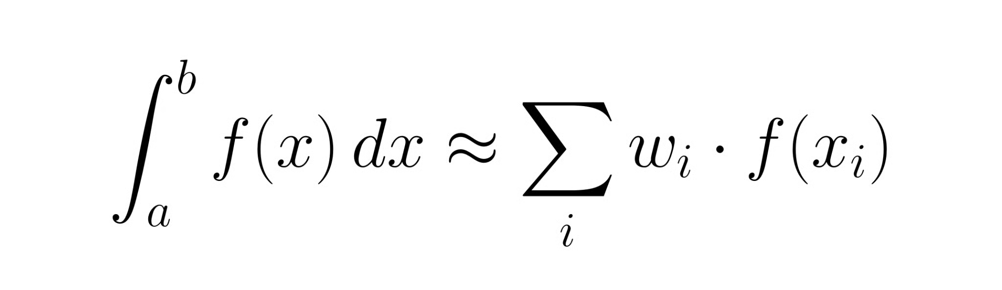
The core idea is a substitution: instead of finding an exact antiderivative, you sample the function f(x) at a set of points called nodes, multiply each value by an associated weight, and sum the results:

The terms quadrature and numerical integration mean essentially the same thing. Quadrature tends to show up in more mathematical contexts; numerical integration is the everyday term in scientific computing.

How Numerical Quadrature Works

Every quadrature rule operates on an interval [a, b]. Within that interval, it selects a set of nodes xᵢ and assigns each one a weight wᵢ. The approximation is the weighted sum above. What differs between methods is where the nodes go and how the weights are assigned. That's it. The trapezoidal rule, Simpson's rule, and Gaussian quadrature are all variations on this same template.

Approximation error is the gap between the weighted sum and the true integral. Every method introduces some, and how fast that error shrinks as you add more nodes (or make intervals smaller) is what separates a good method from a great one. Keep this framing in mind: choosing a quadrature method is really choosing how to spend your function evaluations.

Common Quadrature Methods

The methods below go from most intuitive to most sophisticated.

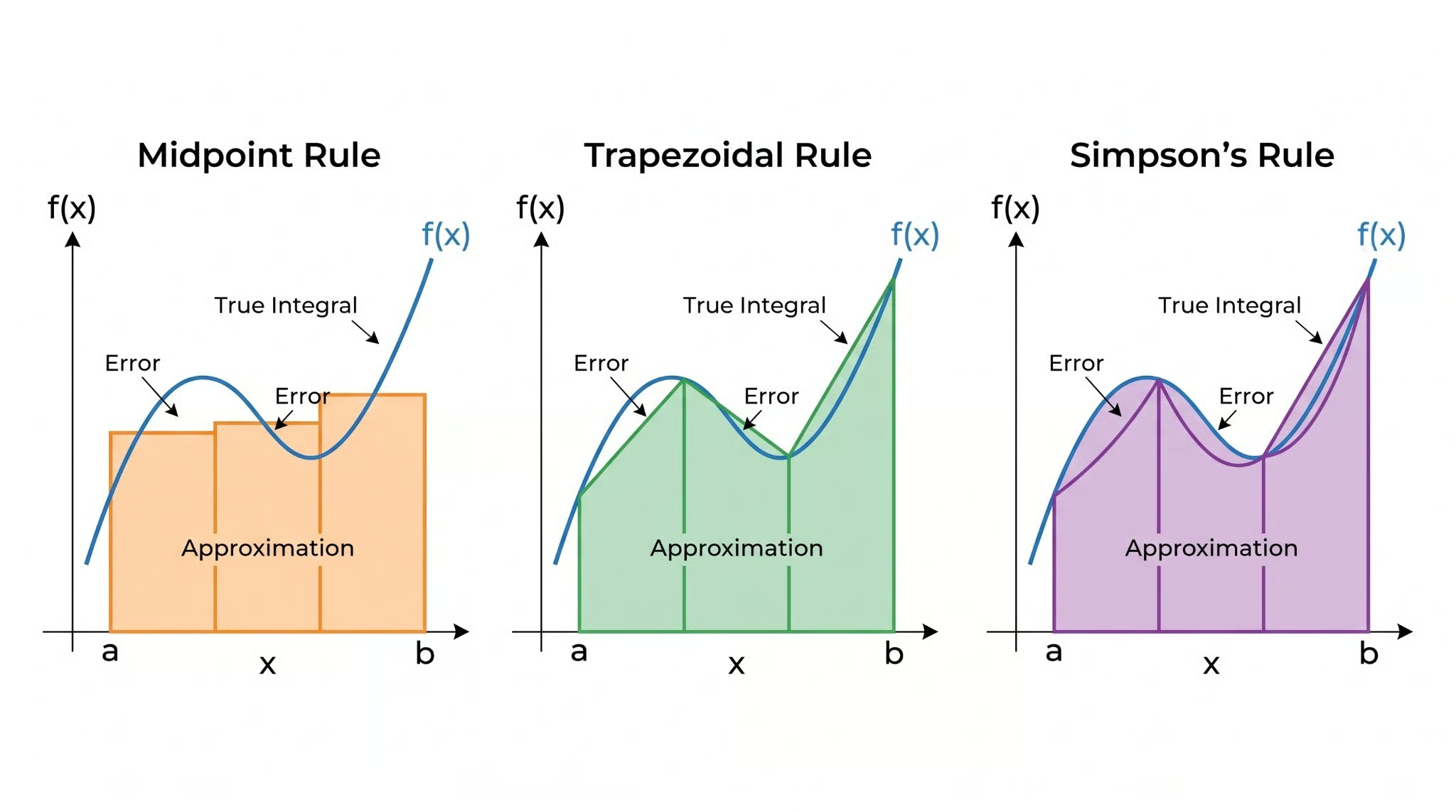Visual comparison of Midpoint, Trapezoidal, and Simpson's integration rules. Image by Author.

Midpoint rule

Take the midpoint of [a, b], evaluate f there, and multiply by the width (b − a). The assumption is that the function value at the center represents the average across the entire interval.

It sounds almost too simple, and for a single interval, it is. But here's the first surprise: the midpoint rule is exact for constant and linear functions, and its error scales as O(h³) per interval where h = b − a. That's actually better than the trapezoidal rule on smooth functions, which tends to catch people off guard.

Trapezoidal rule

Use both endpoints instead of just the center. Connect them with a straight line and compute the area of the resulting trapezoid: (b − a) · [f(a) + f(b)] / 2. Exact for linear functions, with O(h³) error per interval, the same order as the midpoint rule, though with a larger constant.

The trapezoidal rule is probably the most widely taught quadrature method, which has given it an outsized reputation. For well-behaved functions it's decent. But composite Simpson's rule almost always does better for the same number of evaluations.

Simpson's rule

Fit a quadratic polynomial through three points: the two endpoints and the midpoint. Integrate that polynomial exactly:

The extra evaluation at the center costs one additional function call, but the payoff is real: Simpson's rule is exact for polynomials up to degree three, and error per interval scales as O(h⁵), two orders better than the trapezoidal rule. For smooth functions, this is usually the first method worth reaching for.

Gaussian quadrature

Here's where things get genuinely interesting. The midpoint, trapezoidal, and Simpson rules all use evenly spaced nodes. Gaussian quadrature asks a different question: what if we chose both the node locations and the weights to maximize accuracy?

With n nodes, Gaussian quadrature (specifically the Gauss-Legendre variant) can integrate any polynomial of degree up to 2n − 1 exactly. Two nodes gives you exactness for cubics; five nodes handles degree-9 polynomials. The nodes are the roots of Legendre polynomials, and they cluster toward the endpoints of the interval rather than sitting at evenly spaced positions. The extra accuracy comes from letting the nodes move, not from where they happen to land. Their clustering near the endpoints is a byproduct of the math, and we’ll see why below.

Here's how all four methods compare:

Composite Quadrature Methods

Applying a rule once across the full interval [a, b] usually isn't enough. The standard fix: split the interval into n equal subintervals of width h = (b − a)/n and apply the basic rule to each one.

Composite midpoint and trapezoidal rules

For the composite trapezoidal rule, evaluate f at n+1 evenly spaced points and sum n trapezoids. Total error drops to O(h²). Halve h, and the error falls by a factor of four. The composite midpoint rule follows the same logic and has the same global error order.

Composite Simpson's rule

The composite version requires an even number of subintervals. Evaluate f at n+1 points and get O(h⁴) global error. Halving h reduces error by a factor of sixteen. That's why composite Simpson's rule is often the default when you need moderate accuracy on a smooth function.

The Python code below shows how the approximation tightens as you add subintervals for ∫[0 to π] sin(x) dx (exact value: 2.0):

import numpy as np

def composite_simpson(func, lower, upper, num_intervals):
    """Approximate integral using composite Simpson's rule."""
    if num_intervals % 2 != 0:
        raise ValueError("num_intervals must be even")
    nodes = np.linspace(lower, upper, num_intervals + 1)
    values = func(nodes)
    h = (upper - lower) / num_intervals
    weights = np.ones(num_intervals + 1)
    weights[1:-1:2] = 4   # odd-indexed interior points
    weights[2:-2:2] = 2   # even-indexed interior points
    return (h / 3) * np.dot(weights, values)

exact = 2.0
for n in [4, 8, 16, 32]:
    approx = composite_simpson(np.sin, 0, np.pi, n)
    print(f"n={n:3d}: approx={approx:.10f}, error={abs(approx - exact):.2e}")

With just 32 intervals, the error drops below 10⁻⁶. That’s O(h⁴) convergence.

Gaussian Quadrature

The idea behind Gaussian quadrature deserves more than a table entry.

Why evenly spaced nodes aren't always optimal

When nodes sit at evenly spaced points, you're spending evaluation budget in a way that may not match the difficulty of the integrand. Some regions need more resolution; others waste evaluations on flat stretches. Gaussian quadrature sidesteps this by choosing nodes that are provably optimal for the polynomial degree you can integrate exactly.

For n nodes, the Gauss-Legendre rule selects the n roots of the nth Legendre polynomial Pₙ(x) as nodes, then computes weights so that any polynomial of degree ≤ 2n − 1 is integrated without error. In practice, numpy.polynomial.legendre.leggauss(n) returns both. The nodes cluster toward the endpoints of [−1, 1], the standard reference interval, where polynomial interpolation error tends to be largest and where extra sampling density pays off most.

When to use it

Gaussian quadrature is at its best when you have a smooth, analytic function and need high accuracy with few evaluations. Five Gauss-Legendre points can outperform composite Simpson's rule with dozens of intervals on well-behaved integrands. But it's poorly suited to functions with kinks, discontinuities, or data available only at fixed evenly-spaced points. In those cases, the carefully chosen node placement works against you.

Quadrature Error and Accuracy

No numerical method gets a free pass on error. Two distinct sources affect every quadrature result, and understanding both is essential for knowing when to trust your answer.

Sources of error include:

• Discretization error (also called truncation error) is the gap between the exact integral and what your quadrature rule returns in perfect arithmetic. This is what the O(hᵏ) formulas capture. It shrinks as you add more points or reduce interval width.
• Floating-point error is a different problem. Summing many small quantities in finite-precision arithmetic introduces rounding that doesn't shrink with h and can actually grow. With composite rules using thousands of subintervals, you may hit a floor where floating-point noise dominates and adding intervals stops helping. For most scientific computing tasks, you'll hit your desired tolerance well before that floor. But it exists.

Function smoothness, interval width, and method choice all feed into discretization error. A rough function with sharp features needs more intervals or an adaptive approach.

Adaptive Quadrature

A uniform grid wastes evaluations when the integrand is smooth in most places but complicated in a few.

How it works

Apply a quadrature rule to an interval, then apply a higher-order rule (or the same rule on two halves) and compare. The difference estimates local error. If it's below tolerance, accept the interval. If not, split it and recurse on each half. Repeat until every subinterval meets the tolerance.

The efficiency gain over uniform refinement can be large when the integrand has isolated features: a narrow spike, a kink, rapid oscillation surrounded by smooth territory. Adaptive methods concentrate evaluations exactly where the function demands them.

scipy.integrate.quad()

In Python, scipy.integrate.quad() implements adaptive Gaussian quadrature (specifically QUADPACK's DQAGSE algorithm). Pass your function and limits; get back the estimate and an error bound. For most one-dimensional integrals, this is the right tool, no manual tuning required.

from scipy import integrate
import numpy as np

# Integrate a function with a peak near x=0.5
def peaked_func(x):
    return np.exp(-100 * (x - 0.5)**2)

result, error_bound = integrate.quad(peaked_func, 0, 1)
print(f"Estimate: {result:.10f}")
print(f"Error bound: {error_bound:.2e}")

quad() handles this narrow peak cleanly. A uniform Simpson's rule would need hundreds of subintervals to match it.

How to Choose a Quadrature Method

Start with scipy.integrate.quad() for one-dimensional integrals in Python unless you have a reason not to. It's adaptive, accurate, and well-tested. Everything below is relevant when you're implementing something yourself, working in a language without a good adaptive library, or optimizing for a specific case.

• Smooth, analytic functions with a known formula: Gaussian quadrature gives the most accuracy per evaluation. If you need moderate accuracy and simplicity, composite Simpson's rule is a solid default.
• Functions with kinks or discontinuities: Evenly spaced methods (trapezoidal, Simpson's) tend to outperform Gaussian quadrature here, because fixed node placement isn't disrupted by irregularity. Split the integration interval at the known discontinuity and handle each piece separately.
• Data at fixed, evenly-spaced points: Gaussian quadrature is off the table. You can't evaluate the function at arbitrary nodes, so use composite trapezoidal or composite Simpson's rule instead.
• Higher-dimensional integrals: Quadrature runs into the curse of dimensionality quickly. With n points per dimension and d dimensions, you need nᵈ total evaluations. Ten dimensions with ten points each is 10¹⁰ evaluations, which isn't happening. Monte Carlo scales much better above roughly five dimensions, so that's where the switch happens.

Quadrature vs. Related Numerical Methods

Quadrature doesn’t exist in a vacuum. It helps to see where it sits relative to the other tools you’re likely considering.

Quadrature vs. analytical integration

Analytical integration finds an exact antiderivative; quadrature approximates a number. If an exact antiderivative exists and you can find it, use it. Quadrature earns its place when exact integration is impossible or impractical.

Quadrature vs. Monte Carlo integration

Both approximate definite integrals, but differently. Quadrature is deterministic: it evaluates f at fixed, pre-chosen nodes, with convergence tied to function smoothness and node count. Monte Carlo draws random samples and averages them, with error scaling as O(1/√N) regardless of dimension. That's slower convergence in low dimensions, but it's dimension-independent, which makes it the practical choice above roughly five dimensions.

Quadrature vs. interpolation

Some quadrature rules, Simpson's rule included, work by fitting a polynomial through evaluation points and integrating it exactly. But the goal differs from interpolation. Interpolation reconstructs the function; quadrature just wants a number. The polynomial is a tool, not the output.

Conclusion

What I find satisfying about quadrature is how much mileage you get from a single organizing idea. Every method here, midpoint rule, trapezoidal, Simpson's, Gaussian, is really just a different answer to the same question: given a budget of function evaluations, where do you put them, and how do you weigh them?

Fitting better polynomials through evaluation points drives down error fast. Shifting to optimally chosen nodes squeezes out even more accuracy from the same budget. Adaptive methods then bring everything together, routing evaluations to wherever the function actually needs them.

In Python, scipy.integrate.quad() is the right default for 1D problems. Everything else in this article is for when you need to understand what's happening under the hood, or when you're implementing something yourself. If you want to keep building numerical skills with SciPy, take our Introduction to Optimization in Python course.