Gaussian Elimination: A Method to Solve Systems of Equations

Gaussian elimination is one of the most fundamental algorithms in linear algebra for solving systems of linear equations. Named after German mathematician Carl Friedrich Gauss, this method transforms a system of equations into an equivalent, simpler form by performing a sequence of operations on its matrix representation.

This article will explore how Gaussian elimination works, implement it in Python, and examine its applications in data science and numerical computing. By understanding this algorithm, we’ll gain insight into a fundamental technique that underlies many computational methods used in data analysis.

What Is Gaussian Elimination?

Gaussian elimination is an algorithm for solving systems of linear equations by systematically transforming the augmented matrix of the system into row echelon form (REF). This transformation preserves the solution set while making it easier to find the values of the variables.

A matrix is in row echelon form when:

• All rows consisting entirely of zeros are at the bottom of the matrix
• The leading entry (first nonzero element) of each nonzero row is to the right of the leading entry of the row above it
• All elements below a leading entry are zeros

To achieve row echelon form, we use three types of elementary row operations:

• Row swapping: Exchange two rows
• Row scaling: Multiply all elements in a row by a nonzero constant
• Row addition: Replace one row with the sum of itself and a multiple of another row

Additionally, it’s important to distinguish between Gaussian elimination and Gauss-Jordan elimination:

• Gaussian elimination transforms the matrix to row echelon form, requiring back-substitution to find variable values
• Gauss-Jordan elimination continues the process to reduce row echelon form (RREF), where all leading entries are 1 and all other entries in each leading entry’s column are 0

While Gauss–Jordan elimination provides a more direct solution, Gaussian elimination is generally more efficient for large systems, especially when combined with back-substitution and techniques such as LU decomposition.

Step-by-Step Breakdown of the Gaussian Elimination Algorithm

Let’s walk through the Gaussian elimination process using a simple example. Consider the following system of linear equations:

System of linear equations. Image by Author.

Step 1: Create the augmented matrix

First, we represent the system as an augmented matrix, combining the coefficient matrix with the constants:

Augmented matrix. Image by Author.

Step 2: Forward elimination

We’ll now perform elementary row operations to transform the matrix into row echelon form.

Make the first element of the first column a pivot and eliminate all elements below it:

• Add 3/2 × Row 1 to Row 2:

Add 3/2 × Row 1 to Row 2. Image by Author.

• Add Row 1 to Row 3:

Add Row 1 to Row 3. Image by Author.

Move to the second column and eliminate all elements below the pivot:

• Multiply Row 2 by 2 to make the pivot 1:

Multiply Row 2 by 2. Image by Author.

• Subtract 2 × Row 2 from Row 3:

Subtract 2 × Row 2. Image by Author.

Make the pivot in the third row positive:

• Multiply Row 3 by -1:

Multiply Row 3 by -1. Image by Author.

The matrix is now in row echelon form.

Step 3: Back-substitution

Now we can find the values of our variables through back-substitution:

From Row 3: 

          z = -1

From Row 2: 

          y + z = 2,

          so y + (-1) = 2,

          which gives y = 3

From Row 1: 

          2x + y - z = 8,

          so 2x + 3 - (-1) = 8,

          which gives 2x = 4,

          so x = 2

Therefore, the solution is x = 2, y = 3, z = -1.

While we apply the Gaussian elimination to this example, the steps remain the same for another linear system of equations.

Implementation of Gaussian Elimination in Python

While we can write the algorithm using basic Python, NumPy’s vectorized operations make the implementation both cleaner and significantly faster. 

For educational purposes, understanding the underlying algorithm is valuable, but for production use, leveraging optimized libraries is recommended. Having already understood the underlying algorithm in the previous section, we will now delve into the implementation using optimized libraries in Python.

NumPy-based implementation

NumPy provides the numpy.linalg.solve() function, which implements a highly optimized solution for systems of linear equations:

import numpy as np

# Define the coefficient matrix A and constant vector b
A = np.array([[2, 1, -1],
             [-3, -1, 2],
             [-2, 1, 2]], dtype=float)
b = np.array([8, -11, -3], dtype=float)

# Solve the system Ax = b
x = np.linalg.solve(A, b)

print("Solution:", x)

In the code above, we define the coefficient matrix A, along with the constant vector b, are same as the augmented matrix we created in step 1 of the Gaussian elimination example above. 

We use the numpy.linalg.solve()function to arrive at the solution and print the output as seen below:

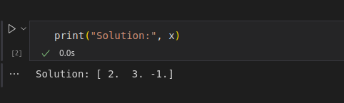
Solution using code implementation. Image by Author.

This implementation uses LAPACK under the hood, which applies LU decomposition (a variant of Gaussian elimination) optimized for numerical stability and performance.

Handling special cases

When implementing Gaussian elimination, you’ll encounter several special cases that require careful handling:

• Singular matrices: If the determinant of your coefficient matrix is zero or very close to zero, the system either has no solution or infinitely many solutions. NumPy’s linalg.solve() function raises a LinAlgError in this case.

• Numerical stability: With floating-point arithmetic, rounding errors can accumulate and lead to inaccurate results. Partial pivoting, where the largest element in a column is selected as the pivot, helps mitigate this issue.

• Overdetermined or underdetermined systems: When the number of equations doesn’t match the number of variables, you can use numpy.linalg.lstsq() instead, which finds the least-squares solution.

For large systems with many zeros, SciPy’s sparse matrix solvers can be orders of magnitude faster than dense solvers:

from scipy.sparse import csr_matrix
from scipy.sparse.linalg import spsolve

# For large sparse matrices
A_sparse = csr_matrix(A)
x = spsolve(A_sparse, b)

While understanding the algorithm’s mechanics is valuable, in practice, leveraging NumPy and SciPy’s optimized implementations allows you to solve linear systems efficiently and reliably without reinventing the wheel.

Where Gaussian Elimination Is Used

Gaussian elimination extends far beyond theoretical mathematics and finds numerous practical applications across various fields of science, engineering, and data analysis. 

Here are some of the most important real-world applications of this fundamental algorithm:

• Linear regression: In data science, Gaussian elimination is used to solve the normal equations that arise when finding the best-fit parameters in linear regression models. This enables analysts to make predictions based on historical data.
• Network analysis: Engineers use Gaussian elimination to solve for unknown currents or voltages in electrical circuits by applying Kirchhoff’s laws, which generate systems of linear equations that must be solved simultaneously.
• Matrix inversion: Gaussian elimination forms the basis for computing matrix inverses, which are essential in transformations, statistical analyses, and solving complex mathematical problems in machine learning algorithms.
• Numerical integration: When implementing advanced numerical methods such as implicit Euler or Runge-Kutta integration schemes, Gaussian elimination is used to solve the resulting systems of equations, ensuring stability in simulations of dynamic systems.

By understanding these applications, we can see how a single mathematical technique can serve as the backbone for many of the tools used daily by data scientists, engineers, and researchers.

Conclusion

This article explored the fundamental algorithm of Gaussian elimination for solving systems of linear equations by transforming matrices into row echelon form. We also learned how to implement this technique in Python using NumPy’s optimized functions, and we understood its practical applications in linear regression, network analysis, matrix inversion, and numerical methods. 

To deepen your knowledge of linear algebra and its applications in data science, consider enrolling in our Linear Algebra course, where you’ll explore more advanced concepts and implementations of these fundamental techniques.