SQLAlchemy Tutorial With Examples

What is SQLAlchemy?

SQLAlchemy is the Python SQL toolkit that allows developers to access and manage SQL databases using Pythonic domain language. You can write a query in the form of a string or chain Python objects for similar queries. Working with objects provides developers flexibility and allows them to build high-performance SQL-based applications. 

In simple words, it allows users to connect databases using Python language, run SQL queries using object-based programming, and streamline the workflow. 

Install SQLAlchemy

It is fairly easy to install the package and get started with coding. 

You can install SQLAlchemy using the Python Package Manager (pip):

pip install sqlalchemy

In case, you are using the Anaconda distribution of Python, try to enter the command in conda terminal:

conda install -c anaconda sqlalchemy

Let’s check if the package is successfully installed:

>>> import sqlalchemy
>>> sqlalchemy.__version__
'1.4.41'

Excellent, we have successfully installed SQLAlchemy version 1.4.41. 

Getting Started

In this section, we will learn to connect SQLite databases, create table objects, and use them to run the SQL query. 

Connecting the database

We will be using the European Football SQLite database from Kaggle, and it has two tables: divisions and matchs.

First, we will create SQLite engine objects using ‘create_object’ and pass the location address of the database. Then, we will create a connection object by connecting the engine. We will use the ‘conn’ object to run all types of SQL queries.

from sqlalchemy as db
engine = db.create_engine("sqlite:///european_database.sqlite")

conn = engine.connect() 

If you want to connect PostgreSQL, MySQL, Oracle, and Microsoft SQL Server databases, check out engine configuration for smooth connectivity to the server. 

This SQLAlchemy tutorial assumes that you understand the fundamentals of Python and SQL. If not, then it is perfectly ok. You can take SQL Fundamentals and Python Fundamentals skill track to build a strong base.                                   

Accessing the table

To create a table object, we need to provide table names and metadata. You can produce metadata using SQLAlchemy’s `MetaData()` function.

metadata = db.MetaData() #extracting the metadata
division= db.Table('divisions', metadata, autoload=True, 
autoload_with=engine) #Table object

Let’s print the “divisions” metadata. 

print(repr(metadata.tables['divisions']))

The metadata contains the table name, column names with the type, and schema. 

Table('divisions', MetaData(), Column('division', TEXT(), table=<divisions>), 
Column('name', TEXT(), table=<divisions>), Column('country', TEXT(), 
table=<divisions>), schema=None)

Let’s use the table object “division” to print column names. 

print(division.columns.keys())

The table consists of a division, name, and country columns. 

['division', 'name', 'country']

Simple SQL query

Now comes the fun part. We will use the table object to run the query and extract the results. 

In the code below, we are selecting all of the columns for the “division” table. 

query = division.select() #SELECT * FROM divisions
print(query)

Note: you can also write the select command as ‘db.select([division])’

To view the query, print the query object, and it will show the SQL command. 

SELECT divisions.division, divisions.name, divisions.country
FROM divisions

SQL query result

We will now execute the query using the connection object and extract the first five rows. 

• fetchone(): it will extract a single row at a time.
• fetchmany(n): it will extract the n number of rows at a time.
• fetchall(): it will extract all of the rows.  

exe = conn.execute(query) #executing the query
result = exe.fetchmany(5) #extracting top 5 results
print(result)

The result shows the first five rows of the table. 

[('B1', 'Division 1A', 'Belgium'), ('D1', 'Bundesliga', 'Deutschland'), ('D2', '2. Bundesliga', 'Deutschland'), ('E0', 'Premier League', 'England'), ('E1', 'EFL Championship', 'England')]

Python SQLAlchemy Examples

In this section, we will look at various SQLAlchemy examples for creating tables, inserting values, running SQL queries, data analysis, and table management. 

You can follow along or check out this DataLab workbook. It contains a database, source code, and results. 

Creating Tables

First, we will create a new database called “datacamp.sqlite”. The create_engine will create a new database automatically if there is no database with the same name. So, creating and connecting are pretty much similar.

After that, we will connect the database and create a metadata object. 

We will use SQLAlchmy’s Table function to create a table called “Student”

It consists of columns:

• Id: Integer and primary key
• Name: String and non-nullable 
• Major: String and default = “Math”
• Pass: Boolean and default =True 

We have created the structure of the table. Let’s add it to the database using `metadata.create_all(engine)`.

engine = db.create_engine('sqlite:///datacamp.sqlite')
conn = engine.connect()
metadata = db.MetaData()

Student = db.Table('Student', metadata,
              db.Column('Id', db.Integer(),primary_key=True),
              db.Column('Name', db.String(255), nullable=False),
              db.Column('Major', db.String(255), default="Math"),
              db.Column('Pass', db.Boolean(), default=True)
              )

metadata.create_all(engine) 

Insert one

To add a single row, we will first use `insert` and add the table object. After that, use `values` and add values to the columns manually. It works similarly to adding arguments to Python functions.   

Finally, we will execute the query using the connection to execute the function.

query = db.insert(Student).values(Id=1, Name='Matthew', Major="English", Pass=True)
Result = conn.execute(query)

Let’s check if we add the row to the “Student” table by executing a select query and fetching all the rows. 

output = conn.execute(Student.select()).fetchall()
print(output)

We have successfully added the values. 

[(1, 'Matthew', 'English', True)]

Insert many

Adding values one by one is not a practical way of populating the database. Let’s add multiple values using lists. 

1. Create an insert query for the Student table.
2. Create a list of multiple rows with column names and values.
3. Execute the query with a second argument as values_list. 

query = db.insert(Student)
values_list = [{'Id':'2', 'Name':'Nisha', 'Major':"Science", 'Pass':False},
              {'Id':'3', 'Name':'Natasha', 'Major':"Math", 'Pass':True},
              {'Id':'4', 'Name':'Ben', 'Major':"English", 'Pass':False}]
Result = conn.execute(query,values_list)

To validate our results, run the simple select query.

output = conn.execute(db.select([Student])).fetchall()
print(output)

The table now contains more rows. 

[(1, 'Matthew', 'English', True), (2, 'Nisha', 'Science', False), (3, 'Natasha', 'Math', True), (4, 'Ben', 'English', False)]

Simple SQL Query with SQLAlchemy

Instead of using Python objects, we can also execute SQL queries using String. 

Just add the argument as a String to the `execute` function and view the result using `fetchall`.

output = conn.execute("SELECT * FROM Student")
print(output.fetchall())

Output:

[(1, 'Matthew', 'English', 1), (2, 'Nisha', 'Science', 0), (3, 'Natasha', 'Math', 1), (4, 'Ben', 'English', 0)]

You can even pass more complex SQL queries. In our case, we are selecting the Name and Major columns where the students have passed the exam. 

output = conn.execute("SELECT Name, Major FROM Student WHERE Pass = True")
print(output.fetchall())

Output:

[('Matthew', 'English'), ('Natasha', 'Math')]

Using SQLAlchemy API

In the previous sections, we have been using simple SQLAlchemy API/Objects. Let’s dive into more complex and multi-step queries.

In the example below, we will select all columns where the student's major is English.  

query = Student.select().where(Student.columns.Major == 'English')
output = conn.execute(query)
print(output.fetchall())

Output:

[(1, 'Matthew', 'English', True), (4, 'Ben', 'English', False)]

Let’s apply AND logic to the WHERE query. 

In our case, we are looking for students who have an English major, and they have failed.  

Note: not equal to ‘!=’ True is False. 

query = Student.select().where(db.and_(Student.columns.Major == 'English', Student.columns.Pass != True))
output = conn.execute(query)
print(output.fetchall())

Only Ben has failed the exam with an English major. 

[(4, 'Ben', 'English', False)]

Using a similar table, we can run all kinds of commands, as shown in the table below. 

You can copy and paste these commands to test the results on your own. Check out the DataLab workbook if you get stuck in any of the given commands. 

To learn about other functions and commands, check out SQL Statements and Expressions API official documentation.

Output to Pandas DataFrame

Data scientists and analysts appreciate pandas dataframes and would love to work with them. In this part, we will learn how to convert an SQLAlchemy query result into a pandas dataframe. 

First, execute the query and save the results. 

query = Student.select().where(Student.columns.Major.in_(['English','Math']))
output = conn.execute(query)
results = output.fetchall()

Then, use the DataFrame function and provide the SQL results as an argument. Finally, add the column names using the result first-row `results[0]` and `.keys()`

Note: you can provide any valid row to extract the names of the columns using `keys()`

data = pd.DataFrame(results)
data.columns = results[0].keys()
data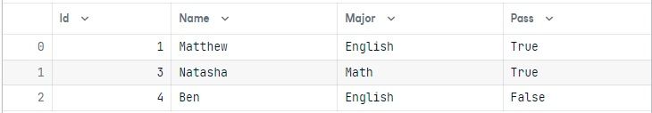

Data Analytics With SQLAlchemy

In this part, we will connect the European football database and perform complex queries and visualize the results.  

Connecting two tables

As usual, we will connect the database using the `create_engine` and `connect` functions.

In our case, we will be joining two tables, so we have to create two table objects: division and match.  

engine = create_engine("sqlite:///european_database.sqlite")
conn = engine.connect()
metadata = db.MetaData()
division = db.Table('divisions', metadata, autoload=True, autoload_with=engine)
match = db.Table('matchs', metadata, autoload=True, autoload_with=engine)

Running complex query

1. We will select both division and match columns.
2. Join them using a common column: division.division and match.Div.
3. Select all columns where the division is E1 and the season is 2009.
4. Order the result by HomeTeam.

You can even create more complex queries by adding additional modules.

Note: to auto-join two table you can also use:  `db.select([division.columns.division,match.columns.Div])`

query = db.select([division,match]).\
select_from(division.join(match,division.columns.division == match.columns.Div)).\
where(db.and_(division.columns.division == "E1", match.columns.season == 2009 )).\
order_by(match.columns.HomeTeam)
output = conn.execute(query)
results = output.fetchall()

data = pd.DataFrame(results)
data.columns = results[0].keys()
data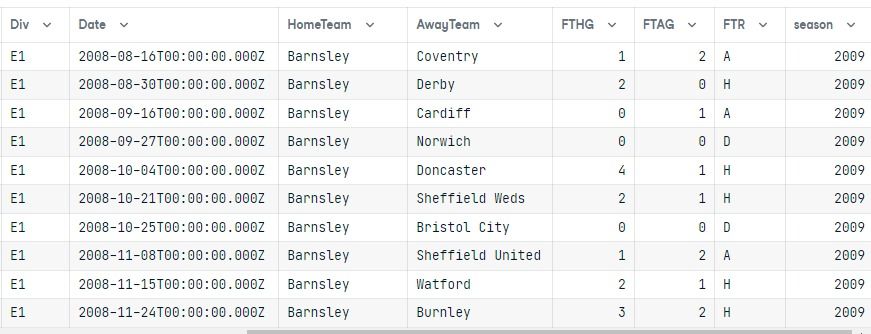

After executing the query, we converted the result into a pandas dataframe. 

Both tables are joined, and the results only show the E1 division for the 2009 season ordered by the HomeTeam column. 

Data Visualization

Now that we have a dataframe, we can visualize the results in the form of a bar chart using Seaborn. 

We will:

1. Set the theme to “whitegrid”
2. Resize the visualization size to 15X6
3. Rotate x-axis ticks to 90
4. Set color palates to “pastels”
5. Plot a bar chart of "HomeTeam" v.s "FTHG" with the color Blue.
6. Plot a bar chart of "HomeTeam" v.s "FTAG" with the color Red.
7. Display the legend on the upper left.
8. Remove the x and y labels. 
9. Despine left and bottom.

The main purpose of this part is to show you how you can use the output of the SQL query and create amazing data visualization. 

import seaborn as sns
import matplotlib.pyplot as plt
sns.set_theme(style="whitegrid")

f, ax = plt.subplots(figsize=(15, 6))
plt.xticks(rotation=90)
sns.set_color_codes("pastel")
sns.barplot(x="HomeTeam", y="FTHG", data=data,
            label="Home Team Goals", color="b")

sns.barplot(x="HomeTeam", y="FTAG", data=data,
            label="Away Team Goals", color="r")
ax.legend(ncol=2, loc="upper left", frameon=True)
ax.set(ylabel="", xlabel="")
sns.despine(left=True, bottom=True)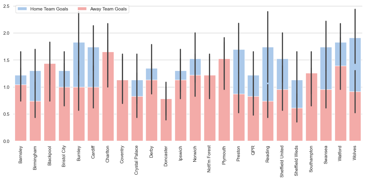

Saving Results to CSV

After converting the query result to pandas dataframe, you can simply use the '.to_csv' function with the file name. 

output = conn.execute("SELECT * FROM matchs WHERE HomeTeam LIKE 'Norwich'")
results = output.fetchall()


data = pd.DataFrame(results)
data.columns = results[0].keys()

Avoid adding a column called “Index” by using `index=False`.

data.to_csv("SQl_result.csv",index=False)

CSV file to SQL Table

In this part, we will convert the Stock Exchange Data CSV file to an SQL table. 

First, connect to the datacamp sqlite database.

engine = create_engine("sqlite:///datacamp.sqlite")

Then, import the CSV file using the read_csv function. In the end, use the `to_sql` function to save the pandas dataframe as an SQL table.  

Primarily, the `to_sql` function requires connection and table name as an argument. You can also use `if_exisits` to replace an existing table with the same name and `index` to drop the index column. 

df = pd.read_csv('Stock Exchange Data.csv')
df.to_sql(con=engine, name="Stock_price", if_exists='replace', index=False)
>>> 2222

To validate the results, we need to connect the database and create a table object. 

conn = engine.connect()
metadata = db.MetaData()
stock = db.Table('Stock_price', metadata, autoload=True, autoload_with=engine)

Then, execute the query and display the results.

query = stock.select()
exe = conn.execute(query)
result = exe.fetchmany(5)
for r in result:
    print(r)

As you can see, we have successfully transferred all the values from the CSV file to the SQL table. 

('HSI', '1986-12-31', 2568.300049, 2568.300049, 2568.300049, 2568.300049, 2568.300049, 0, 333.87900637)
('HSI', '1987-01-02', 2540.100098, 2540.100098, 2540.100098, 2540.100098, 2540.100098, 0, 330.21301274)
('HSI', '1987-01-05', 2552.399902, 2552.399902, 2552.399902, 2552.399902, 2552.399902, 0, 331.81198726)
('HSI', '1987-01-06', 2583.899902, 2583.899902, 2583.899902, 2583.899902, 2583.899902, 0, 335.90698726)
('HSI', '1987-01-07', 2607.100098, 2607.100098, 2607.100098, 2607.100098, 2607.100098, 0, 338.92301274)

SQL Table Management

Updating the values in table

Updating values is straightforward. We will use the update, values, and where functions to update the specific value in the table. 

table.update().values(column_1=1, column_2=4,...).where(table.columns.column_5 >= 5)

In our case, we have changed the “Pass” value from False to True where the name of the student is “Nisha”.  

Student = db.Table('Student', metadata, autoload=True, autoload_with=engine)
query = Student.update().values(Pass = True).where(Student.columns.Name == "Nisha")
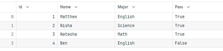
results = conn.execute(query)

To validate the results, let’s execute a simple query and display the results in the form of a pandas dataframe. 

output = conn.execute(Student.select()).fetchall()
data = pd.DataFrame(output)
data.columns = output[0].keys()
data

We have successfully changed the “Pass” value to True for the student name “Nisha”.

Delete the records

Deleting the rows is similar to updating. It requires delete and where function. 

table.delete().where(table.columns.column_1 == 6)

In our case, we are deleting the record of the student named “Ben”.

Student = db.Table('Student', metadata, autoload=True, autoload_with=engine)
query = Student.delete().where(Student.columns.Name == "Ben")
results = conn.execute(query)

To validate the results, we will run a quick query and display the results in the form of a dataframe. As you can see, we have deleted the row containing the student name ”Ben”.

output = conn.execute(Student.select()).fetchall()
data = pd.DataFrame(output)
data.columns = output[0].keys()
data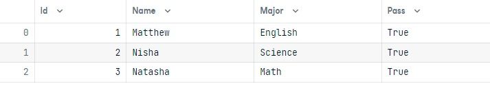

Dropping tables

If you are using SQLite, dropping the table will throw an error “database is locked“. Why? Because SQLite is a very light version. It can only perform one function at a time. Currently, it is executing a select query. We need to close all of the execution before deleting the table. 

results.close()
exe.close()

After that, use metadata’s drop_all function and select a table object to drop the single table. You can also use the `Student.drop(engine)` command to drop a single table.

metadata.drop_all(engine, [Student], checkfirst=True)

If you don’t specify any table for the drop_all function. It will drop all of the tables in the database. 

metadata.drop_all(engine)

Conclusion 

The SQLAlchemy tutorial covers various functions of SQLAlchemy, from connecting the database to modifying tables, and if you are interested in learning more, try completing the Introduction to Databases in Python interactive course. You will learn about the basics of relational databases, filtering, ordering, and grouping. Furthermore, you will learn about advanced SQLAlchemy functions for data manipulation.  

If you are finding any issues in following the tutorial, head over to the DataLab workbook and compare your code with it. You can also make a copy of the workbook and run it right inside DataLab.