SymPy: A Complete Guide to Symbolic Mathematics in Python

If you’ve ever wanted Python to perform and express algebraic operations like a mathematician, SymPy is your answer.

SymPy stands for Symbolic Python, and it’s a library built to perform symbolic computations, which means that it can expand, simplify, differentiate, and solve equations symbolically, just like you would do on paper.  An important extension is that mathematical expressions with unevaluated variables are left in symbolic form. For instance, the square root of eight will be represented as 2*sqrt(2), instead of approximating it to 2.828.   

Some of the major advantages of SymPy are that it’s open source, written completely in Python, and that it offers compatibility with other Python libraries. 

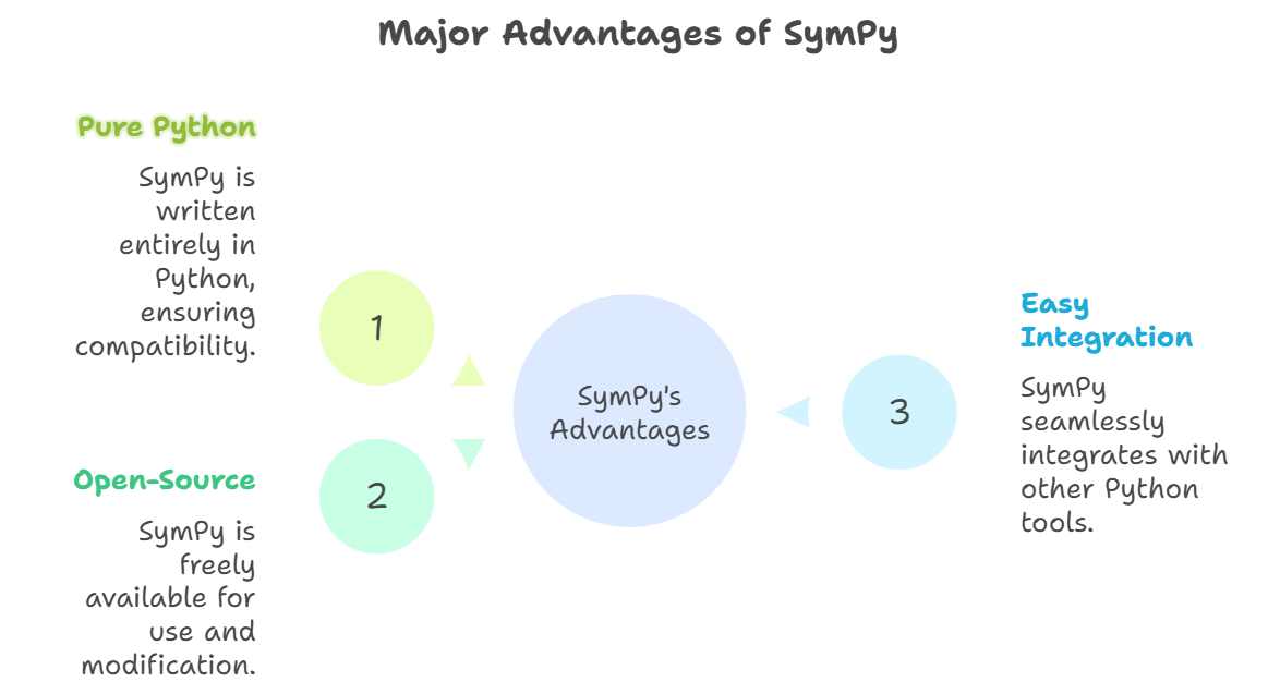
Major advantages of Sympy. Source: Image by Napkin AI

Brief History of SymPy

SymPy began with a simple idea: to make symbolic computation accessible to everyone.

It was started in 2006 by Ondřej Čertík, a student at the University of Nevada. He wanted to make a lightweight, flexible symbolic math library in pure Python so that people wouldn't have to deal with the complexities of big computer algebra systems like Maple or Mathematica. 

Between 2007 and 2010, SymPy grew rapidly as it participated in Google Summer of Code, during which major core modules such as simplification, solving, and calculus were significantly expanded. 

By around 2012, SymPy had matured to the point where it was integrated into SageMath, signalling its recognition as a reliable symbolic backend within the broader scientific Python ecosystem. As of today, SymPy has evolved beyond its usage in algebra into advanced domains including physics, geometry, combinatorics, code generation, and performance-oriented compilation tools.

Getting Started with SymPy

Before exploring SymPy’s magic, let’s set it up correctly.

Installation and setup

The easiest way to install SymPy, which also is the recommended method, is using pip:

pip install sympy

If you’re using Conda, the command is:

conda install sympy

Alternatively, you can install directly from source (useful for contributors):

git clone https://github.com/sympy/sympy.git

If you are wondering about dependencies: SymPy runs entirely in Python and doesn’t depend on external libraries. Optional packages like mpmath can be installed for arbitrary precision arithmetic:

pip install mpmath

Verifying installation

To confirm the installation, open Python and type:

import sympy
print(sympy.__version__)

1.14.0

The output shows the installed version of the package.  You can now test the package with a simple expression:

from sympy import symbols

# Define x as a symbolic variable
x = symbols('x')

print((x + 2)**2)

(x + 2)**2

As for troubleshooting:

• If you see ModuleNotFoundError, re-run pip install sympy.

• For version conflicts, upgrade pip: pip install --upgrade pip

Also, what is good to know: If you think there’s a bug or you would like to request a feature, you can also open an issue ticket. For detailed exploration on installation methods, check out the official documentation.

Basic usage

SymPy provides an interactive environment where you can manipulate algebraic expressions symbolically.

from sympy import symbols, expand

#define x and y as symbolic variables
x, y = symbols('x y')

# create an algebraic expression
expr = (x + y)**2

expanded = expand(expr)
print(expanded)

x**2 + 2*x*y + y**2

The printed output above x**2 + 2*x*y + y**2 is the fully expanded form, demonstrating how SymPy performs exact symbolic algebra rather than numerical computation.

Core Features and Functionalities

The core functionalities are built around symbolic computation — which means working with functions, equations, and expressions as symbols instead of numbers.

Arithmetic operations

You can treat symbolic variables like algebraic ones. Also, the functions can move from one form to another as demonstrated in the code below. 

By using expand() for distribution and factor() for reverse simplification, SymPy transforms between expanded and factored forms of an algebraic expression.

from sympy import symbols, expand, factor

# Define symbolic variables x and y
x, y = symbols('x y')

# Create an algebraic expression
expr = (x + y)**2

# Expand the expression to its full polynomial form
print(expand(expr))  

# Factor the expanded polynomial back into its compact form
print(factor(x**2 + 2*x*y + y**2)) 

x**2 + 2*x*y + y**2
(x + y)**2

Simplification techniques

Simplification is central to symbolic computation. There is a general function in Sympy, called simplify(),  that is used to simplify rational, trigonometric, or algebraic expressions easily.

from sympy import simplify, trigsimp, sin, cos

# Create a trigonometric expression
expr = sin(x)**2 + cos(x)**2

# General simplification — recognizes that sin²x + cos²x = 1
print(simplify(expr)) 

# Trigonometric-specific simplification — also simplifies to 1
print(trigsimp(expr)) 

The output in both the simplify() and trigsimp() functions above comes out to be one. 

Calculus operations

SymPy is great for calculus because it lets you do differentiation, integration, limits, and even series expansions all symbolically, just like solving by hand but with perfect accuracy.

Differentiation

To take derivatives, use the diff() function.

from sympy import diff

# Define a symbolic polynomial expression
f = x**3 + 2*x**2 + x

# Compute the derivative of the expression with respect to x
df = diff(f, x)
print(df)

3*x**2 + 4*x + 1

Integration

The code below computes the indefinite integral of the symbolic expression f with respect to the variable x using SymPy’s integrate() function. The resulting antiderivative is then printed.

from sympy import integrate

# Compute the indefinite integral of the expression f with respect to x
integral = integrate(f, x)
print(integral)

x**4/4 + 2*x**3/3 + x**2/2

Limits

The calculation for the limit is a classical calculus operation, which can be performed using SymPy’s limit() function. The syntax is: limit(f(x), x, x0).  For example, the code below calculates the limit of the expression sin(x)/x as x approaches zero and prints the exact result, one. 

from sympy import limit, sin

# Compute the limit of sin(x)/x as x approaches 0 
limit_expr = limit(sin(x)/x, x, 0)
print(limit_expr) 

Series expansion

The series() function can be used to compute the Taylor or power series expansion of a mathematical expression around a specified point.

from sympy import series, exp

# Generate the Taylor series expansion of e^x around 0 up to 5 terms
print(series(exp(x), x, 0, 5))

1 + x + x**2/2 + x**3/6 + x**4/24 + O(x**5)

Summations

The summation() function in SymPy performs exact symbolic summation over a certain range, just like the sigma notation in maths.

from sympy import summation, symbols

# Compute the symbolic sum of 1/n^2 from n = 1 to 5
n = symbols('n')
print(summation(1/n**2, (n, 1, 5)))  

5269/3600

Solving equations

SymPy makes it easy to solve symbolic equations - not only the simple algebraic ones, but also systems of equations, differential equations, and even Diophantine equations, which only have integers as solutions. 

It has powerful solvers like 

• solve() for algebraic equations, 

• linsolve() for linear systems, and 

• dsolve() for differential equations that give exact solutions whenever possible. 

Algebraic equations

from sympy import Eq, solve
# Define and solve the equation x^2 - 4 = 0 symbolically
eq = Eq(x**2 - 4, 0)

print(solve(eq, x)) 

[-2, 2]

Systems of equations

from sympy import linsolve, symbols

# Solve a system of linear equations:
# x + y = 5  and  x - y = 1
x, y = symbols('x y')
sol = linsolve([x + y - 5, x - y - 1], (x, y))

print(sol) # Outputs the solution as a set (x, y)

{(3, 2)}

Differential equations

from sympy import Function, dsolve

# Define y as a symbolic function of x
y = Function('y')

# Define a second-order differential equation
diff_eq = Eq(y(x).diff(x, 2) - y(x), 0)

# Solve the differential equation symbolically
print(dsolve(diff_eq))

Eq(y(x), C1*exp(-x) + C2*exp(x))

Matrix operations

SymPy is a great tool for linear algebra as it supports symbolic matrices. You can easily work with matrices and perform mathematical operations like addition and multiplication, just like you would in regular algebra. 

from sympy import Matrix

# Define symbolic matrices A and B
A = Matrix([[1, 2], [x, 3]])
B = Matrix([[x], [4]])

# Perform matrix multiplication
print(A * B)

Matrix([[x + 8], [x**2 + 12]])

Advanced operations

SymPy also lets you calculate important matrix properties like determinants, inverses, eigenvalues, and eigenvectors symbolically, giving you exact answers. 

# Compute the determinant of matrix A
A.det()      

# Compute the inverse of matrix A
A.inv()      

# Compute the eigenvalues of matrix A
A.eigenvals() 

{2 - sqrt(2*x + 1): 1, sqrt(2*x + 1) + 2: 1}

Plotting capabilities

SymPy isn’t limited to symbolic computation — it also supports visualization of mathematical expressions. Using the built-in plotting utilities, you can generate 2D and even 3D plots of symbolic functions with few lines of code. 

For instance, the code below generates a 2D plot:  

from sympy.plotting import plot


# Plot the function x^2 over the range -5 to 5
plot(x**2, (x, -5, 5))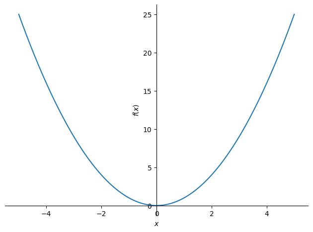

2D Plot generated using SymPy. 

For generating 3D plots, you can use the plot3d() function as shown below.

from sympy.plotting import plot3d
from sympy import sin

# Generate a 3D surface plot of the function sin(x*y) over the specified x and y ranges
plot3d(sin(x*y), (x, -5, 5), (y, -5, 5))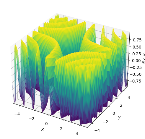

3D Plotting Capability of SymPy

And if you need more control or styling, SymPy can also integrate with Matplotlib to enable fully customizable visualizations. For more advanced visualizations, read our tutorial on Plotly Shapes.

Advanced Capabilities

SymPy goes far beyond basic algebra — it extends into polynomials, combinatorics, and even physics.

Polynomial manipulation

You can define and manipulate polynomials easily. The code below creates a polynomial object from the expression; and then prints its degree, factorized form with coefficients using SymPy’s Poly() function. 

from sympy import Poly

# Create a symbolic polynomial in variable x
p = Poly(x**3 - 3*x**2 + x - 3, x)

# Print the degree of the polynomial (highest power of x)
print(p.degree())  

# Print the factorized form of the polynomial along with coefficients
print(p.factor_list())  

3
(1, [(Poly(x - 3, x, domain='ZZ'), 1), (Poly(x**2 + 1, x, domain='ZZ'), 1)])

For complex polynomial systems, Gröbner bases are supported, which are a simplified and standardized version of a system of polynomial equations, making them easier to solve. 

For example, the code below computes the Gröbner basis for the polynomial system [x*y - 1, y - x], which means it rewrites the equations into a simpler, more structured form that’s easier to solve. The output shows that the system is equivalent to the cleaner equations x = y and y² = 1, which can now be directly solved.

from sympy import groebner, symbols

# Define x and y as symbolic variables
x, y = symbols('x y')

# Compute the Gröbner basis for the system of polynomial equations
print(groebner([x*y - 1, y - x], x, y))

GroebnerBasis([x - y, y**2 - 1], x, y, domain='ZZ', order='lex')

Combinatorics, discrete math, and number theory

SymPy has several utilities that enable it to handle combinatorial and number-theoretic problems. 

For example, in the code below:

• The binomial(5, 2) function calculates the number of ways to choose 2 items from 5 (a combination problem), 

• factorial(6) computes 6!, a common operation in permutations. 

• isprime(19) checks if 19 is a prime number, and 

• factorint(100) returns its exact prime factorization as {2: 2, 5: 2}. 

from sympy import binomial, factorial, isprime, factorint
print(binomial(5, 2))   # 10
print(factorial(6))     # 720
print(isprime(19))      # True
print(factorint(100))   # {2: 2, 5: 2}

10
720
True
{2: 2, 5: 2}

10
720
True
{2: 2, 5: 2}

Together, these functions illustrate how SymPy handles discrete maths with ease and accuracy. You can also work with partitions, permutations, and combinations directly.

Geometry and physics applications

SymPy is not just meant for algebra and calculus; it also offers special modules for geometry and physics. 

In the geometry module, you can define mathematical objects like points, lines, circles, and polygons. Using symbols, you may also obtain equations of lines, intersections, distances, and midpoints. 

For example, to make two points and draw a line between them, just do this:

from sympy import Point, Line, Circle

# Define two points and create a line passing through them
A, B = Point(0, 0), Point(1, 1)
L = Line(A, B)

# Print the symbolic equation of the line
print(L.equation())  

-x + y

In addition to its geometry capabilities, SymPy provides a very useful physics module. With this module, you can model classical mechanics, quantum systems, units, and sizes.  This is true whether you're using meters per second to find speed or solving motion equations with symbols. 

from sympy.physics.units import meter, second

# Define a symbolic physical quantity: velocity = 10 meters per second
velocity = 10 * meter / second
print(velocity)

10*meter/second

Printing and LaTeX output

SymPy allows you to print symbolic expressions in multiple formats, including:

• Human-friendly pretty printing 
• Unicode-based output, and 
• LaTeX, which is the standard formatting language used in research papers and scientific documentation. 

You can use functions like pprint() to make your equations look neat and professional in a Jupyter notebook or while producing a report. You can even use latex() to get them ready for a research paper. It saves you the trouble of having to format everything yourself.

from sympy import pprint, latex, symbols

# Define x and y as symbolic variables
x, y = symbols('x y')

# Now you can perform symbolic math operations
expr = (x+y)**3

# Pretty print to the console
pprint(expr)

# Print the LaTeX string
print(latex(expr))

     3
(x + y) 
\left(x + y\right)^{3}

Code Generation and Performance Optimization

While SymPy excels at symbolic computation, it also allows you to convert symbolic expressions into optimized executable code for high-performance numerical use.

The code below uses SymPy’s codegen() utility to automatically generate C language code from a symbolic expression, making it ready for use in embedded applications.

from sympy.utilities.codegen import codegen

# Generate C code for the symbolic function and save it as 'output'
codegen(("f", x**2 + 1), "C", "output")

[('output.c',
  '/******************************************************************************\n *                      Code generated with SymPy 1.14.0                      *\n *                                                                            *\n *              See http://www.sympy.org/ for more information.               *\n *                                                                            *\n *                       This file is part of \'project\'                       *\n ******************************************************************************/\n#include "output.h"\n#include <math.h>\n\ndouble f(double x) {\n\n   double f_result;\n   f_result = pow(x, 2) + 1;\n   return f_result;\n\n}\n'),
 ('output.h',
  "/******************************************************************************\n *                      Code generated with SymPy 1.14.0                      *\n *                                                                            *\n *              See http://www.sympy.org/ for more information.               *\n *                                                                            *\n *                       This file is part of 'project'                       *\n ******************************************************************************/\n\n\n#ifndef PROJECT__OUTPUT__H\n#define PROJECT__OUTPUT__H\n\ndouble f(double x);\n\n#endif\n\n")]

Lambdify

The lambdify() function converts symbolic expressions to fast numeric Python functions. For example, the code below uses lambdify to convert the symbolic expression stored under the object, f, into a fast NumPy-compatible Python function. When evaluated on the array [1, 2, 3], it returns [4, 9, 16]. 

from sympy import lambdify
import numpy as np

# Convert the symbolic expression into a fast numerical function using NumPy
f = lambdify(x, x**2 + 2*x + 1, 'numpy')

# Evaluate the function on a NumPy array
print(f(np.array([1, 2, 3])))

[ 4  9 16]

Performance considerations

Since SymPy is concerned with symbolic accuracy, it can be slower than numeric computations. Having said that, there are a number of ways to improve performance when working with large or complicated expressions. 

For example, you can use lambdify() to turn symbolic expressions into fast numerical functions that work well with NumPy, or you can simplify them before you evaluate them. 

You can speed up heavy computations even more by using techniques like common subexpression elimination, automatic code compilation, and integration with outside tools like Numba or Cython.

SymPy in the Python Ecosystem

SymPy doesn’t work in isolation — it integrates well with other popular tools used in data science, education, and research and fits right in with the larger scientific Python ecosystem.

Integration with other libraries

You can combine SymPy with:

• NumPy/SciPy for high-performance numerics
• Matplotlib for visualization
• Pandas for symbolic data analysis

import numpy as np
from sympy import lambdify

# Convert the symbolic expression x^2 into a fast NumPy-compatible function
f = lambdify(x, x**2, 'numpy')

# Evaluate the function on a NumPy array from 0 to 4
print(f(np.arange(5)))

[ 0  1  4  9 16]

Educational applications

SymPy is widely used in classrooms and self-learning environments because it mirrors the way mathematics is taught on paper — step-by-step and symbolically. In Jupyter Notebooks, students can experiment live with algebra, calculus, or physics equations and see exact symbolic results instead of rough approximations. See Jupyter Notebook Cheat Sheet to get started.

Related projects and integrations

SymPy also connects well with other powerful mathematical tools, such as:

• SageMath — a large-scale math system using SymPy as a backend.
• SymEngine — a faster, C++ reimplementation of SymPy’s core.
• Pyomo — integrates optimization modeling (see Optimizing with Pyomo).

Community, Contribution, and Development

SymPy thrives because of a strong open-source community. A worldwide group of developers, researchers, teachers, and students works on SymPy, making it better and robust day by day. Anyone can help, ask questions, or get involved without needing permission or a corporate membership.

Contribution and development

People who want to help usually fork the repository, make changes, run the test suite with pytest, and then send in a pull request for review.

To make sure that every change is reliable, it goes through a code review process. The project also has a testing framework so that contributors can run tests on their own machines before submitting. 

Reporting bugs and seeking support

For bugs or help:

• File issues on GitHub under SymPy Issues
• Ask on Stack Overflow 
• Join the SymPy Gitter or Mailing list

The more clearly you explain the problem, including the code, what you expected to happen, what actually happened, and what version of SymPy you are using, the faster the community can help. 

Future directions

SymPy is still growing, with work still going on to expand its features, improve its performance, and integrate with AI tools. There are also efforts to make code generation, documentation, and educational use better. New contributors are especially welcome to help with sorting through the bugs and issues, making documentation better, and adding new features for symbolic mathematics.

Conclusion

SymPy is a powerful library that lets you use symbolic math in Python. This makes it useful for education, research, and even engineering work in the real world. It provides an open-source ecosystem, inside of which you can perform various mathematical and algebraic operations and transformations. SymPy is a tool that students, developers, and researchers should look into. So go ahead — open a Jupyter notebook, import sympy, and start exploring. 

You can also refer to the following resources for further reading:

• SciPy Cheat Sheet: Linear Algebra in Python
• SymPy Documentation
• How to Square a Number in Python