Types of Data Plots and How to Create Them in Python

Common Types of Data Plots

Let's start with the most common data plots that are widely used in many fields and can be built in the majority of Python data visualization libraries (except for some very narrowly-specialized ones).

Bar chart

A bar chart is the most common data visualization for displaying the numerical values of categorical data to compare various categories between them. The categories are represented by rectangular bars of the same width and with heights (for vertical bar charts) or lengths (for horizontal bar charts) proportional to the numerical values that they correspond to.

To create a basic bar chart in matplotlib, we use the matplotlib.pyplot.bar() function, as follows:

# Data preparation
penguins_grouped = penguins[['species', 'bill_length_mm']].groupby('species').mean().reset_index()
​
# Creating a bar chart
plt.bar(penguins_grouped['species'], penguins_grouped['bill_length_mm'])
plt.title('Average penguin bill length by species')
plt.show()

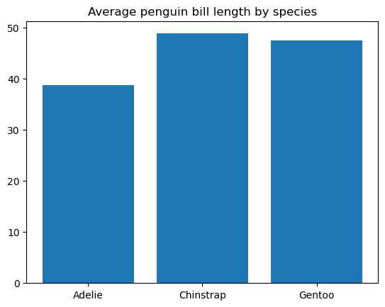
We can further customize the bar width and color, bar edge width and color, add tick labels to the bars, fill the bars with patterns, etc.

As a quick refresher on how to work in matplotlib, take a look at our Matplotlib Cheat Sheet: Plotting in Python.

Line plot

A line plot is a type of data chart that shows a progression of a variable from left to right along the x-axis through data points connected by straight line segments. Most typically, the change of a variable is plotted over time. Indeed, line plots are often used for visualizing time series, as discussed in the tutorial on Matplotlib time series line plots.

We can create a basic line plot in matplotlib by using the matplotlib.pyplot.plot() function, as follows:

# Data preparation
flights_grouped = flights[['year', 'passengers']].astype({'year': 'string'}).groupby('year').sum().reset_index()
​
# Creating a line plot
plt.plot(flights_grouped['year'], flights_grouped['passengers'])
plt.title('Total number of passengers by year')
plt.show()

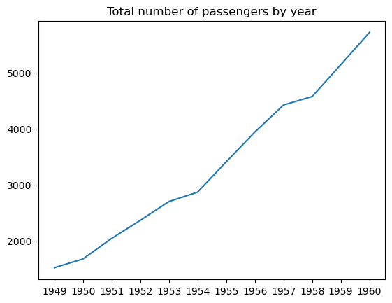
It's possible to adjust the line width, style, color, and transparency, add and customize markers, etc.

The tutorial on Line Plots in MatplotLib with Python provides more explanations and examples on how to create and customize a line plot in matplotlib. To learn how to create and customize a line plot in seaborn, read Python Seaborn Line Plot Tutorial: Create Data Visualizations.

Scatter plot

A scatter plot is a data visualization type that displays the relationships between two variables plotted as data points on the coordinate plane. This type of data plot is used to check if the two variables correlate among themselves, how strong this correlation is, and if there are distinct clusters in the data.

The code below illustrates how to create a basic scatter plot in matplotlib using the matplotlib.pyplot.scatter() function:

# Creating a scatter plot
plt.scatter(penguins['bill_length_mm'], penguins['bill_depth_mm'])
plt.title('Penguin bill length vs. bill depth')
plt.show()

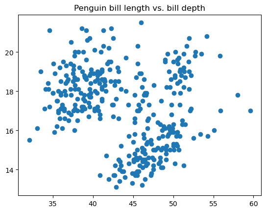
We can adjust the point size, style, color, transparency, edge width, edge color, etc.

You can read more about scatter plots (and not only!) in this tutorial: Data Demystified: Data Visualizations that Capture Relationships.

Histogram

A histogram is a type of data plot that represents the frequency distribution of the values of a numerical variable. Under the hood, it splits the data into value range groups called bins, counts the number of points related to each bin, and displays each bin as a vertical bar, with the height proportional to the count value for that bin. A histogram can be considered as a specific type of bar charts, only that its adjacent bars are attached without gaps, given the continuous nature of bins.

We can easily build a basic histogram in matplotlib using the matplotlib.pyplot.hist() function:

# Creating a histogram
plt.hist(penguins['bill_length_mm'])
plt.title('Penguin bill length distribution')
plt.show()

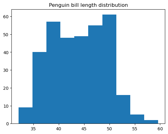
It's possible to customize many things inside this function, including the histogram color and style, the number of bins, the bin edges, the lower and upper range of the bins, whether the histogram is regular or cumulative, etc.

In the tutorial on How to Create a Histogram with Plotly, you can explore another way of creating a histogram in Python.

Box plot

A box plot is a data plot type that shows a set of five descriptive statistics of the data: the minimum and maximum values (excluding the outliers), the median, and the first and third quartiles. Optionally, it can also show the mean value. A box plot is the right choice if you're interested only in these statistics, without digging into the real underlying data distribution.

In the tutorial on 11 Data Visualization Techniques for Every Use-Case with Examples, you'll find, among other things, more granular explanations about what kind of statistical information you can obtain from a box plot.

We can create a basic box plot in matplotlib using the matplotlib.pyplot.boxpot() function, as below:

# Data preparation
penguins_cleaned = penguins.dropna()
​
# Creating a box plot
plt.boxplot(penguins_cleaned['bill_length_mm'])
plt.title('Penguin bill length distribution')
plt.show()

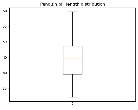
There is plenty of room for customizing a box plot: the box width and orientation, the box and whisker position, the visibility and style of various box plot elements, etc.

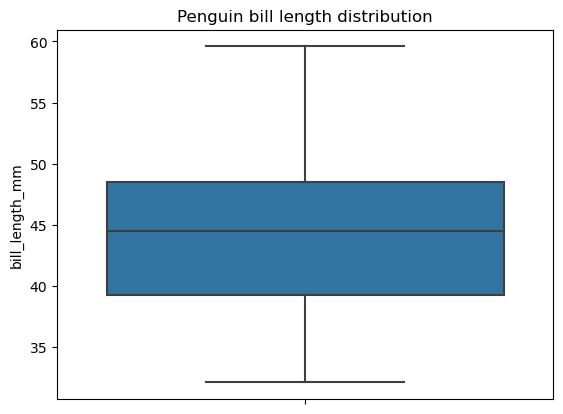
Note that to create a box plot using this function, we need to ensure first that the data doesn't contain missing values. Indeed, in the above example, we dropped the missing values from the data before plotting. For comparison, the Seaborn library doesn't have this limitation and handles missing values behind the scenes, as below:

# Creating a box plot
sns.boxplot(data=penguins, y='bill_length_mm')
plt.title('Penguin bill length distribution')
plt.show()

Pie chart

A pie chart is a type of data visualization represented by a circle divided into sectors, where each sector corresponds to a certain category of the categorical data, and the angle of each sector reflects the proportion of that category as a part of the whole. Unlike bar charts, pie charts are supposed to depict the categories that constitute the whole, e.g., passengers of a ship.

Pie charts have some drawbacks:

• Angles are more difficult to interpret for the human eye than lengths and often can be misleading.
• They are less efficient in the case of five or more categories.
• They can't display more than one set of categorical data. In other words, they can't be grouped, unlike bar charts.
• They don't easily reveal real values.
• They aren't informative when it comes to the categories with a small difference in their values.

Hence, pie charts should be used sparingly and with caution.

To create a basic pie chart in matplotlib, we need to apply the matplotlib.pyplot.pie() function, as follows:

# Data preparation
titanic_grouped = titanic.groupby('class')['pclass'].count().reset_index()
​
# Creating a pie chart
plt.pie(titanic_grouped['pclass'], labels=titanic_grouped['class'])
plt.title('Number of passengers by class')
plt.show()

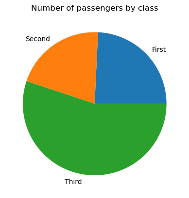
If necessary, we can adjust our pie plot: change the colors of its wedges, add an offset to some wedges (usually very small ones), change the circle radius, customize the format of labels, fill some or all wedges with patterns, etc.

Advanced Types of Data Plots

In this section, we're going to explore various advanced data plots. Some of them represent a fancy variation of common types of data visualizations that we considered in the previous section, others are just stand-alone types.

Grouped bar chart

While a common bar chart is used for displaying the numerical values of a categorical variable by category, a grouped bar chart serves the same purpose but across two categorical variables. Graphically, it means that we have several groups of bars, with each group related to a certain category of one variable and each bar of those groups related to a certain category of the second variable. Grouped bar charts work best when the second variable has no more than three categories. In the opposite case, they become too crowded and hence less helpful.

Like a common bar chart, we can create a grouped bar chart with matplotlib. However, the Seaborn library offers a more convenient functionality of its seaborn.barplot() function for creating such plots. Let's look at an example of creating a basic grouped bar chart for penguin bill length across two categorical variables: species and sex.

# Creating a grouped bar chart
sns.barplot(data=penguins, x='species', y='bill_length_mm', hue='sex')
plt.title('Penguin bill length by species and sex')
plt.show()

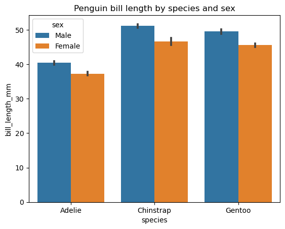
The second categorical variable is introduced through the hue parameter. Other optional parameters of this function allow changing bar orientation, width, and color, the category order, the statistical estimator, etc.

To dive deeper into plotting with Seaborn, consider the following course: Intermediate Data Visualization with Seaborn.

Stacked area chart

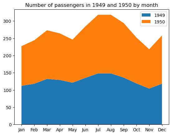
A stacked area chart is an extension of a common area chart (which is simply a line plot with the area below the line colored or filled with a pattern) with multiple areas, each corresponding to a particular variable, stacked on top of each other. Such charts are useful when we need to track both the overall progress of a set of variables and the individual contribution of each variable to this progress. Like line plots, stacked area charts usually reflect the change of variables over time.

It's important to keep in mind the main limitation of stacked area charts: they mostly help capture the general trend but not exact values for the stacked areas.

To build a basic stacked area chart in matplotlib, we use the matplotlib.pyplot.stackplot fuction, as below:

# Data preparation
flights_grouped = flights.groupby(['year', 'month']).mean().reset_index()
flights_49_50 = pd.DataFrame(list(zip(flights_grouped.loc[:11, 'month'].tolist(), flights_grouped.loc[:11, 'passengers'].tolist(), flights_grouped.loc[12:23, 'passengers'].tolist())), columns=['month', '1949', '1950'])
​
# Creating a stacked area chart
plt.stackplot(flights_49_50['month'], flights_49_50['1949'], flights_49_50['1950'], labels=['1949', '1950'])
plt.title('Number of passengers in 1949 and 1950 by month')
plt.legend()
plt.show()

Some customizable properties of this type of graph are the area colors, transparency, filling patterns, line width, style, color, transparency, etc.

Multiple box plot

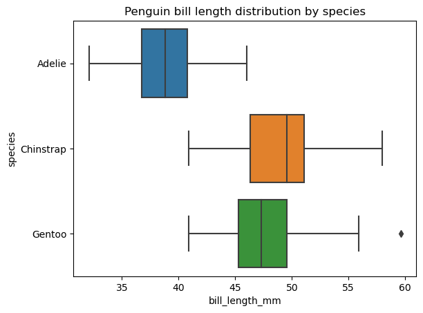
In the section on Common Types of Data Plots, we defined a box pot as a data visualization type that shows a set of five descriptive statistics of the data. Sometimes, we may want to display and compare these statistics separately for each category of a categorical variable. In such cases, we need to plot multiple boxes on the same plot area, which we can easily do with the seaborn.boxplot() function, as follows:

# Creating multiple box plots
sns.boxplot(data=penguins, x='bill_length_mm', y='species')
plt.title('Penguin bill length distribution by species')
plt.show()

It's possible to change the order of the box plots, their orientation, color, transparency, width, the properties of their various elements, add another categorical variable on the plot area, etc.

Violin plot

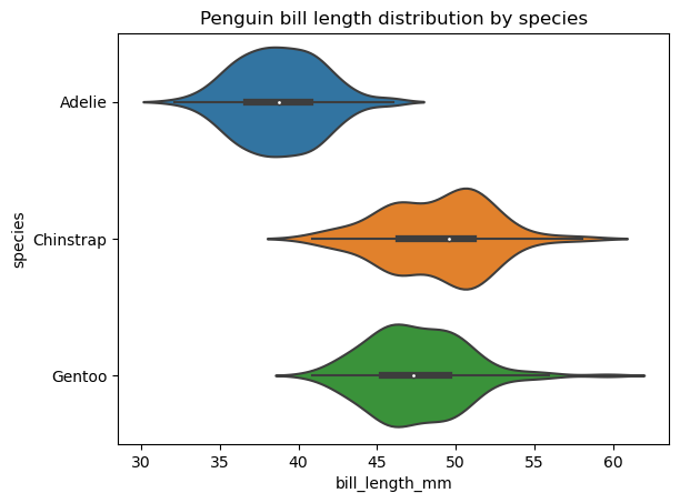
A violin plot is similar to a box plot and displays the same overall statistics of the data, except that it also displays the distribution shape for that data. Like with box plots, we can create a single violin plot for the data in interest or, more often, multiple violin plots, each for a separate category of a categorical variable.

Seaborn provides more room for creating and customizing violin plots than matplotlib. To build a basic violin plot in seaborn, we need to apply the seaborn.violinplot() function, as below:

 Creating a violin plot
sns.violinplot(data=penguins, x='bill_length_mm', y='species')
plt.title('Penguin bill length distribution by species')
plt.show()

We can modify the order of the violins, their orientation, color, transparency, width, the properties of their various elements, extend the distribution past the extreme data points, add another categorical variable on the plot area, select the way the data points are represented in the violin interior, etc.

Heatmap

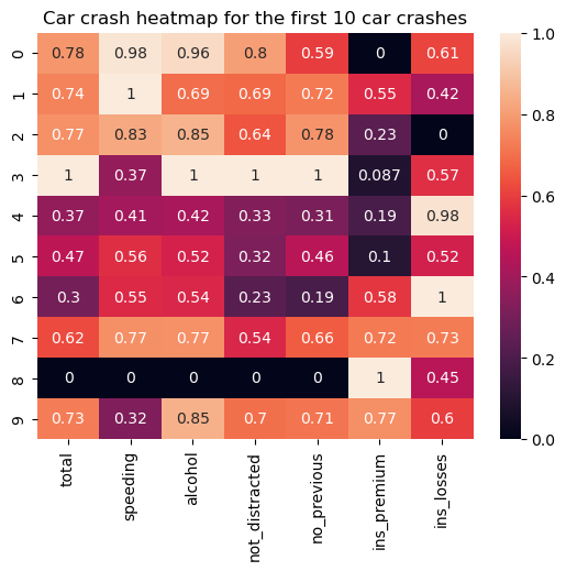
A heatmap is a table-style data visualization type where each numeric data point is depicted based on a selected color scale and according to the data point's magnitude within the dataset. The main idea behind these plots is to illustrate potential hot and cold spots of the data that may require special attention.

In many cases, the data needs some preprocessing before creating a heatmap for them. This usually implies data cleaning and normalization.

The code below shows how to create a basic heatmap (after the necessary data preprocessing) using the seaborn.heatmap() function:

# Data preparation
from sklearn import preprocessing
car_crashes_cleaned = car_crashes.drop(labels='abbrev', axis=1).iloc[0:10]
min_max_scaler = preprocessing.MinMaxScaler()
car_crashes_normalized = pd.DataFrame(min_max_scaler.fit_transform(car_crashes_cleaned.values), columns=car_crashes_cleaned.columns)
​
# Creating a heatmap
sns.heatmap(car_crashes_normalized, annot=True)
plt.title('Car crash heatmap for the first 10 car crashes')
plt.show()

Some possible adjustments may include selecting a colormap, defining the anchoring values, formatting annotations, customizing the separatory lines, applying a mask, etc.

Unconventional Types of Data Plots

Finally, let's take a look at some rarely-used or even lesser-known types of data visualizations. Many of them have at least one analog among more popular types of graphs. However, in some particular cases, these unconventional data visualizations can do a more efficient job than commonly used plots.

Stem plot

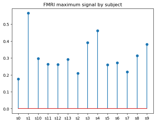
A stem plot is virtually another way to represent a bar chart, only that instead of solid bars, it consists of thin lines with (optional) markers on top of each of them. While a stem plot may seem to be a redundant variation of a bar chart, it's actually its better alternative when it comes to visualizing many categories. The advantage of stem plots over bar charts is that they have an improved data-ink ratio and, hence, enhanced readability.

To create a basic stem plot in matplotlib, we use the matplotlib.pyplot.stem() function, as follows:

# Data preparation
fmri_grouped = fmri.groupby('subject')[['subject', 'signal']].max()
​
# Creating a stem plot
plt.stem(fmri_grouped['subject'], fmri_grouped['signal'])
plt.title('FMRI maximum signal by subject')
plt.show()

We can play with the optional parameters of the function to change the stem orientation and customize the stem, baseline, and marker properties.

Strip and Swarm Plots

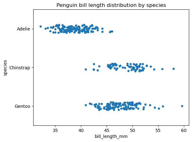
These two very similar types of data visualizations can be regarded as an implementation of a scatter plot for a categorical variable: both strip and swarm plots display the interior of the data distribution, including the sample size and position of individual data points but excluding descriptive statistics. The main difference between these plots is that in a strip plot, the data points can overlap, while in a swarm plot, they cannot. Instead, in a swarm plot, the data points are aligned along the categorical axis.

Keep in mind that both strip and swarm plots can be helpful only for relatively small datasets.

Here is how we can create a strip plot with the seaborn.stripplot() function:

# Creating a strip plot
sns.stripplot(data=penguins, x='bill_length_mm', y='species')
plt.title('Penguin bill length distribution by species')
plt.show()

Now, let's create a swarm plot with the seaborn.swarmplot() function for the same data and observe the difference:

# Creating a swarm plot
sns.swarmplot(data=penguins, x='bill_length_mm', y='species')
plt.title('Penguin bill length distribution by species')
plt.show()

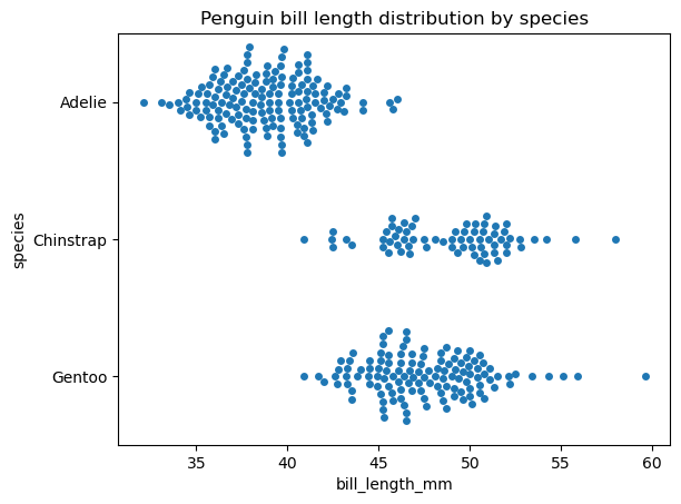
The seaborn.stripplot() and seaborn.swarmplot() functions have very similar syntax. Some customizable properties in both functions are the plot order and orientation and marker properties, such as the marker style, size, color, transparency, etc. It's worth mentioning that regulating marker transparency helps partially fix the point overlapping issue in a strip plot.

Treemap

A treemap is a type of data plot used to visualize the numerical values of the categorical data by category as a set of rectangles placed inside a rectangular frame, with the area of each rectangle proportional to the value of the corresponding category. By their purpose, treemaps are identical to bar charts and pie charts. Like pie charts, they are mostly supposed to depict the categories that constitute the whole. Treemaps can look effective and compelling when there are up to ten categories with a discernible difference in their numerical values.

The disadvantages of treemaps are very similar to those of pie charts:

• Areas are more difficult to interpret for the human eye than lengths and often can be misleading.
• They are less efficient in the case of more than ten categories.
• They can't display more than one set of categorical data. In other words, they can't be grouped, unlike bar charts.
• They don't easily reveal real values.
• They aren't informative when it comes to the categories with a small difference in their values.

We should keep in mind these points and use treemaps sparingly and only when they work best.

To build a treemap in Python, we need first to install and import the squarify library: pip install squarify, then import squarify. The code below creates a basic treemap:

import squarify
​
# Data preparation
diamonds_grouped = diamonds[['cut', 'price']].groupby('cut').mean().reset_index()
​
# Creating a treemap
squarify.plot(sizes=diamonds_grouped['price'], label=diamonds_grouped['cut'])
plt.title('Average diamond price by cut')
plt.show()

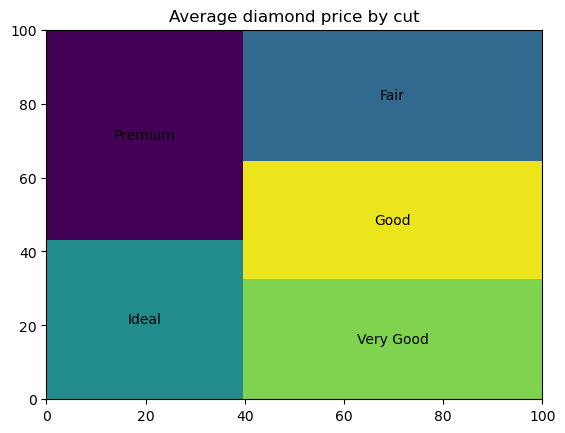
We can customize the colors and transparency of the rectangles, fill them with patterns, adjust the rectangle edge properties, add a small gap between the rectangles, and tune the label text properties.

There is another approach to creating a treemap in Python—by using the plotly library. You can read more about it in the tutorial What is Data Visualization? A Guide for Data Scientists.

Word cloud

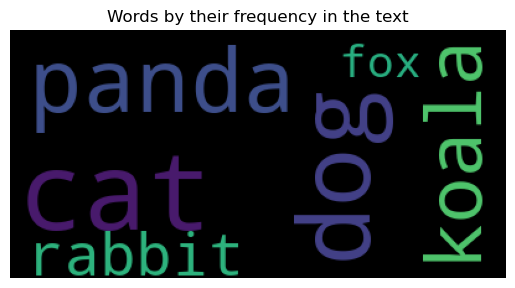
A word cloud is a text data visualization type where the font size of each word corresponds to the frequency of its appearance in an input text. Using word clouds helps find the most important words in a piece of text.

While word clouds are always eye-catching and intuitively understandable for any kind of target audience, we should be aware of some intrinsic limitations of this type of data plots:

• Creating a word cloud often requires a lot of time-consuming data preparation.
• Like the majority of text mining tools, word clouds lack context and can be prone to misinterpretations. For example, they don't capture sarcasm, negation, or illiteral word meaning in a text.
• They don't allow a clear word ranking. This means that we can easily distinguish the most frequent word, the second one, the third, maybe the fourth. Then everything becomes not so easy.
• They don't reveal precise values of word frequencies.
• They create an optical illusion that longer words seem bigger than shorter words of the same frequency.
• Having many vertical words or applying a mask reduces the graph's readability.

An interesting and lesser-known application of word clouds is that we can make them based not on the word frequency but on any other attribute assigned to each word. For example, we can create a dictionary of countries, assign to each country the value of its population, and display this data.

To create a word cloud in Python, we need to use a specialized wordcloud library. First, we need to install it (pip install wordcloud), then import the WordCloud class and stopwords: from wordcloud import WordCloud, STOPWORDS. The following code generates a basic word cloud:

from wordcloud import WordCloud, STOPWORDS
​
text = 'cat cat cat cat cat cat dog dog dog dog dog panda panda panda panda koala koala koala rabbit rabbit fox'
​
# Creating a word cloud
wordcloud = WordCloud().generate(text)
plt.imshow(wordcloud)
plt.title('Words by their frequency in the text')
plt.axis('off')
plt.show()

It's possible to adjust the dimensions of a word cloud, change its background color, assign a colormap for displaying words, set the preference to horizontal words over vertical ones, limit the maximum number of displayed words, update the list of stopwords, limit the font sizes, take into account word collocations, ensure the graph reproducibility, etc.

If you want to learn more about word clouds in Python, here is a great read: Generating WordClouds in Python Tutorial. Also, you can use a free template to practice creating this type of data visualizations: Template: Create a Word Cloud.

Conclusion

In this article, we discussed several types of data plots, their areas of use, their limitations, and how to build and customize them in Python. We started with the most common data visualizations, proceeded with more advanced ones, and then wrapped up with some unconventional but sometimes very helpful types of data plots.

As a brief summary of when to use each of the data plots we’ve covered, you can find our useful Data Visualization Cheat Sheet.

Apart from Python, there are many other tools for creating insightful data visualizations. Below is a selection of beginner-friendly, comprehensive, and exhaustive courses that you can find useful:

• Data Visualization with R
• Data Visualization in Excel
• Data Visualization in Power BI
• Data Visualization in Tableau
• Data Visualization in Spreadsheets