Run and edit the code from this tutorial online
Run codeWhat is a Word Cloud?
Many times you might have seen a cloud filled with lots of words in different sizes, which represent the frequency or the importance of each word. This is called a Tag Cloud or word cloud. For this tutorial, you will learn how to create a word cloud in Python and customize it as you see fit. This tool will be handy for exploring text data and making your report more lively.
Practice generating a WordCloud in Python with this hands-on exercise.
In this tutorial, we will use a wine review dataset from the Wine Enthusiast website to learn:
- How to create a basic word cloud from one to several text documents
- Adjust the color, size, and number of text inside your word cloud
- Mask your word cloud into any shape of your choice
- Mask your word cloud into any color pattern of your choice
When to Use a Word Cloud
It's important to remember that while word clouds are useful for visualizing common words in a text or data set, they're usually only useful as a high-level overview of themes. They're similar to bar blots but are often more visually appealing (albeit at times harder to interpret). Word clouds can be particularly helpful when you want to:
- Quickly identify the most important themes or topics in a large body of text
- Understand the overall sentiment or tone of a piece of writing
- Explore patterns or trends in data that contain textual information
- Communicate the key ideas or concepts in a visually engaging way
However, it's important to keep in mind that word clouds don't provide any context or deeper understanding of the words and phrases being used. Therefore, they should be used in conjunction with other methods for analyzing and interpreting text data.
Prerequisites
To get started making a word cloud in Python, you will need to install some packages below:
The numpy library is one of the most popular and helpful libraries that is used for handling multi-dimensional arrays and matrices. It is also used in combination with the pandas library to perform data analysis.
The Python os module is a built-in library, so you don't have to install it. To read more about handling files with os module, this DataCamp tutorial on reading and writing files in Python will be helpful.
For visualization, matplotlib is a basic library that enables many other libraries to run and plot on its base, including seaborn or wordcloud that you will use in this tutorial. The pillow library is a package that enables image reading. Pillow is a wrapper for PIL - Python Imaging Library. You will need this library to read in image as the mask for the word cloud.
wordcloud can be a little tricky to install. If you only need it for plotting a basic word cloud, then pip install wordcloud or conda install -c conda-forge wordcloud would be sufficient. However, the latest version, with the ability to mask the cloud into any shape of your choice, requires a different method of installation as below:
git clone https://github.com/amueller/word_cloud.git
cd word_cloud
pip install .
Dataset:
This tutorial uses the wine review dataset from Kaggle. This collection is a great dataset for learning with no missing values (which will take time to handle) and a lot of text (wine reviews), categorical, and numerical data.
Creating a Word Cloud in Python: Preparation
Install the necessary libraries
First thing first, you load all the necessary libraries:
# Start with loading all necessary libraries
import numpy as np
import pandas as pd
from os import path
from PIL import Image
from wordcloud import WordCloud, STOPWORDS, ImageColorGenerator
import matplotlib.pyplot as plt
% matplotlib inlinec:\intelpython3\lib\site-packages\matplotlib\__init__.py:
import warnings
warnings.filterwarnings("ignore")
If you have more than 10 libraries, organize them by sections (such as basic libs, visualization, models, etc.). Using comments in the code will make your code clean and easy to follow.
Load the data into the dataframe
Now, using pandas read_csv to load in the dataframe. Notice the use of index_col=0 meaning we don't read in row name (index) as a separate column.
# Load in the dataframe
df = pd.read_csv("data/winemag-data-130k-v2.csv", index_col=0)
# Looking at first 5 rows of the dataset
df.head()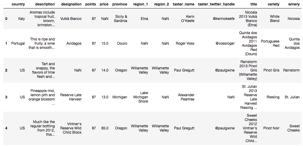
You can printout some basic information about the dataset using print() combined with .format() to have a nice printout.
print("There are {} observations and {} features in this dataset. \n".format(df.shape[0],df.shape[1]))

print("There are {} types of wine in this dataset such as {}... \n".format(len(df.variety.unique()),
                                                                           ", ".join(df.variety.unique()[0:5])))

print("There are {} countries producing wine in this dataset such as {}... \n".format(len(df.country.unique()),
                                                                                      ", ".join(df.country.unique()[0:5])))
There are 129971 observations and 13 features in this dataset.
There are 708 types of wine in this dataset such as White Blend, Portuguese Red, Pinot Gris, Riesling, Pinot Noir...
There are 44 countries producing wine in this dataset such as Italy, Portugal, US, Spain, France...df[["country", "description","points"]].head()| country | description | points | |
|---|---|---|---|
| 0 | Italy | Aromas include tropical fruit, broom, brimston... | 87 |
| 1 | Portugal | This is ripe and fruity, a wine that is smooth... | 87 |
| 2 | US | Tart and snappy, the flavors of lime flesh and... | 87 |
| 3 | US | Pineapple rind, lemon pith and orange blossom ... | 87 |
| 4 | US | Much like the regular bottling from 2012, this... | 87 |
Create groups to compare features
To make comparisons between groups of a feature, you can use groupby() and compute summary statistics.
With the wine dataset, you can group by country and look at either the summary statistics for all countries' points and price or select the most popular and expensive ones.
# Groupby by country
country = df.groupby("country")

# Summary statistic of all countries
country.describe().head()
This selects the top 5 highest average points among all 44 countries:
country.mean().sort_values(by="points",ascending=False).head()| country | points | price |
|---|---|---|
| England | 91.581081 | 51.681159 |
| India | 90.222222 | 13.333333 |
| Austria | 90.101345 | 30.762772 |
| Germany | 89.851732 | 42.257547 |
| Canada | 89.369650 | 35.712598 |
Plot the data
You can plot the number of wines by country using the plot method of Pandas DataFrame and Matplotlib. If you are not familiar with Matplotlib, take a quick look at our Matplotlib tutorial.
plt.figure(figsize=(15,10))
country.size().sort_values(ascending=False).plot.bar()
plt.xticks(rotation=50)
plt.xlabel("Country of Origin")
plt.ylabel("Number of Wines")
plt.show()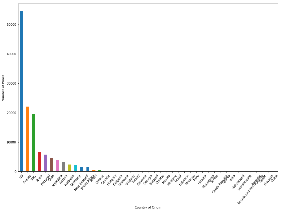
Among 44 countries producing wine, the US has more than 50,000 types in the wine review dataset, twice as much as the next one in the rank, France - the country famous for its wine. Italy also produces a lot of quality wine, having nearly 20,000 wines open to review.
Examine the data
Let's now take a look at the plot of all 44 countries by its highest-rated wine, using the same plotting technique as above:
plt.figure(figsize=(15,10))
country.max().sort_values(by="points",ascending=False)["points"].plot.bar()
plt.xticks(rotation=50)
plt.xlabel("Country of Origin")
plt.ylabel("Highest point of Wines")
plt.show()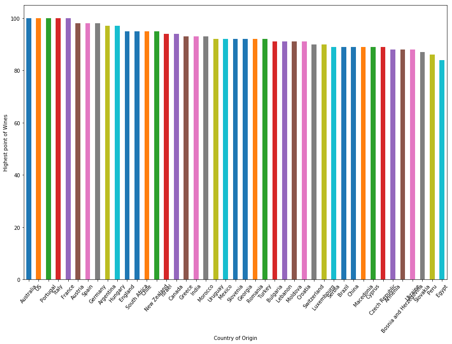
Australia, US, Portugal, Italy, and France all have 100 points wines. If you notice, Portugal ranks 5th and Australia ranks 9th in the number of wines produces in the dataset, and both countries have less than 8000 types of wine.
That's a little bit of data exploration to get to know the dataset that you are using today. Now you will start to dive into the main course of the meal: the word cloud.
Setting up a Basic Word Cloud in Python
Getting started
A word cloud is a technique to show which words are the most frequent in the given text. We can use a Python library to help us with this. The first thing you may want to do before using any functions is to check out the docstring of the function and see all required and optional arguments. To do so, type ?function and run it to get all information.
?WordCloud[1;31mInit signature:[0m [0mWordCloud[0m[1;33m([0m[0mfont_path[0m[1;33m=[0m[1;32mNone[0m[1;33m,[0m [0mwidth[0m[1;33m=[0m[1;36m400[0m[1;33m,[0m [0mheight[0m[1;33m=[0m[1;36m200[0m[1;33m,[0m [0mmargin[0m[1;33m=[0m[1;36m2[0m[1;33m,[0m [0mranks_only[0m[1;33m=[0m[1;32mNone[0m[1;33m,[0m [0mprefer_horizontal[0m[1;33m=[0m[1;36m0.9[0m[1;33m,[0m [0mmask[0m[1;33m=[0m[1;32mNone[0m[1;33m,[0m [0mscale[0m[1;33m=[0m[1;36m1[0m[1;33m,[0m [0mcolor_func[0m[1;33m=[0m[1;32mNone[0m[1;33m,[0m [0mmax_words[0m[1;33m=[0m[1;36m200[0m[1;33m,[0m [0mmin_font_size[0m[1;33m=[0m[1;36m4[0m[1;33m,[0m [0mstopwords[0m[1;33m=[0m[1;32mNone[0m[1;33m,[0m [0mrandom_state[0m[1;33m=[0m[1;32mNone[0m[1;33m,[0m [0mbackground_color[0m[1;33m=[0m[1;34m'black'[0m[1;33m,[0m [0mmax_font_size[0m[1;33m=[0m[1;32mNone[0m[1;33m,[0m [0mfont_step[0m[1;33m=[0m[1;36m1[0m[1;33m,[0m [0mmode[0m[1;33m=[0m[1;34m'RGB'[0m[1;33m,[0m [0mrelative_scaling[0m[1;33m=[0m[1;36m0.5[0m[1;33m,[0m [0mregexp[0m[1;33m=[0m[1;32mNone[0m[1;33m,[0m [0mcollocations[0m[1;33m=[0m[1;32mTrue[0m[1;33m,[0m [0mcolormap[0m[1;33m=[0m[1;32mNone[0m[1;33m,[0m [0mnormalize_plurals[0m[1;33m=[0m[1;32mTrue[0m[1;33m,[0m [0mcontour_width[0m[1;33m=[0m[1;36m0[0m[1;33m,[0m [0mcontour_color[0m[1;33m=[0m[1;34m'black'[0m[1;33m)[0m[1;33m[0m[0m
[1;31mDocstring:[0m
Word cloud object for generating and drawing.
Parameters
----------
font_path : string
Font path to the font that will be used (OTF or TTF).
Defaults to DroidSansMono path on a Linux machine. If you are on
another OS or don't have this font; you need to adjust this path.
width : int (default=400)
Width of the canvas.
height : int (default=200)
Height of the canvas.
prefer_horizontal : float (default=0.90)
The ratio of times to try horizontal fitting as opposed to vertical.
If prefer_horizontal < 1, the algorithm will try rotating the word
if it doesn't fit. (There is currently no built-in way to get only
vertical words.)
mask : nd-array or None (default=None)
If not None, gives a binary mask on where to draw words. If mask is not
None, width and height will be ignored, and the shape of mask will be
used instead. All white (#FF or #FFFFFF) entries will be considered
"masked out" while other entries will be free to draw on. [This
changed in the most recent version!]
contour_width: float (default=0)
If mask is not None and contour_width > 0, draw the mask contour.
contour_color: color value (default="black")
Mask contour color.
scale : float (default=1)
Scaling between computation and drawing. For large word-cloud images,
using scale instead of larger canvas size is significantly faster, but
might lead to a coarser fit for the words.
min_font_size : int (default=4)
Smallest font size to use. Will stop when there is no more room in this
size.
font_step : int (default=1)
Step size for the font. font_step > 1 might speed up computation but
give a worse fit.
max_words : number (default=200)
The maximum number of words.
stopwords : set of strings or None
The words that will be eliminated. If None, the build-in STOPWORDS
list will be used.
background_color : color value (default="black")
Background color for the word cloud image.
max_font_size : int or None (default=None)
Maximum font size for the largest word. If None, the height of the image is
used.
mode : string (default="RGB")
Transparent background will be generated when mode is "RGBA" and
background_color is None.
relative_scaling : float (default=.5)
Importance of relative word frequencies for font-size. With
relative_scaling=0, only word-ranks are considered. With
relative_scaling=1, a word that is twice as frequent will have twice
the size. If you want to consider the word frequencies and not only
their rank, relative_scaling around .5 often looks good.
.. versionchanged: 2.0
Default is now 0.5.
color_func : callable, default=None
Callable with parameters word, font_size, position, orientation,
font_path, random_state that returns a PIL color for each word.
Overwrites "colormap".
See colormap for specifying a matplotlib colormap instead.
regexp : string or None (optional)
Regular expression to split the input text into tokens in process_text.
If None is specified, ``r"\w[\w']+"`` is used.
collocations : bool, default=True
Whether to include collocations (bigrams) of two words.
.. versionadded: 2.0
colormap : string or matplotlib colormap, default="viridis"
Matplotlib colormap to randomly draw colors from for each word.
Ignored if "color_func" is specified.
.. versionadded: 2.0
normalize_plurals : bool, default=True
Whether to remove trailing 's' from words. If True and a word
appears with and without a trailing 's', the one with trailing 's'
is removed and its counts are added to the version without
trailing 's' -- unless the word ends with 'ss'.
Attributes
----------
``words_`` : dict of string to float
Word tokens with associated frequency.
.. versionchanged: 2.0
``words_`` is now a dictionary
``layout_`` : list of tuples (string, int, (int, int), int, color))
Encodes the fitted word cloud. Encodes for each word the string, font
size, position, orientation, and color.
Notes
-----
Larger canvases will make the code significantly slower. If you need a
large word cloud, try a lower canvas size, and set the scale parameter.
The algorithm might give more weight to the ranking of the words
then their actual frequencies, depending on the ``max_font_size`` and the
scaling heuristic.
[1;31mFile:[0m c:\intelpython3\lib\site-packages\wordcloud\wordcloud.py
[1;31mType:[0m typeYou can see that the only required argument for a WordCloud object is the text, while all others are optional.
Start with a simple input
So let's start with a simple example: using the first observation description as the input for the word cloud. The three steps are:
- Extract the review (text document)
- Create and generate a wordcloud image
- Display the cloud using matplotlib
# Start with one review:
text = df.description[0]

# Create and generate a word cloud image:
wordcloud = WordCloud().generate(text)

# Display the generated image:
plt.imshow(wordcloud, interpolation='bilinear')
plt.axis("off")
plt.show()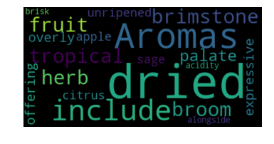
Great! You can see that the first review mentioned a lot about dried flavors and the aromas of the wine.
Changing optional word cloud arguments
Now, change some optional arguments of the word cloud like max_font_size, max_word, and background_color.
# lower max_font_size, change the maximum number of word and lighten the background:
wordcloud = WordCloud(max_font_size=50, max_words=100, background_color="white").generate(text)
plt.figure()
plt.imshow(wordcloud, interpolation="bilinear")
plt.axis("off")
plt.show()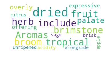
It seems like using max_font_size here might not be a good idea. It makes it more difficult to see the differences between word frequencies. However, brightening the background makes the cloud easier to read.
If you want to save the image, WordCloud provides the function to_file
# Save the image in the img folder:
wordcloud.to_file("img/first_review.png")
<wordcloud.wordcloud.WordCloud at 0x16f1d704978>The result will look like this when you load them in:
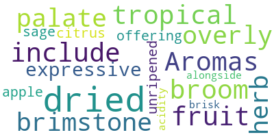
You've probably noticed the argument interpolation="bilinear" in the plt.imshow(). This is to make the displayed image appear more smoothly. For more information about the choice, this interpolation methods for imshow tutorial is a useful resource.
Combining data
So now you'll combine all wine reviews into one big text and create a big fat cloud to see which characteristics are most common in these wines.
text = " ".join(review for review in df.description)
print ("There are {} words in the combination of all review.".format(len(text)))
There are 31661073 words in the combination of all review.
# Create stopword list:
stopwords = set(STOPWORDS)
stopwords.update(["drink", "now", "wine", "flavor", "flavors"])

# Generate a word cloud image
wordcloud = WordCloud(stopwords=stopwords, background_color="white").generate(text)

# Display the generated image:
# the matplotlib way:
plt.imshow(wordcloud, interpolation='bilinear')
plt.axis("off")
plt.show()
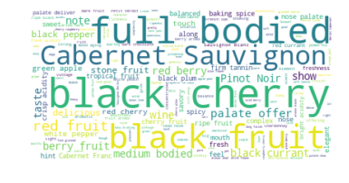
It seems like black cherry and full-bodied are the most mentioned characteristics, and Cabernet Sauvignon is the most popular of them all. This aligns with the fact that Cabernet Sauvignon "is one of the world's most widely recognized red wine grape varieties. It is grown in nearly every major wine-producing country among a diverse spectrum of climates from Canada's Okanagan Valley to Lebanon's Beqaa Valley".[1]
Word cloud visualization in Python
Now, let's pour these words into a cup (or even a bottle) of wine!
In order to create a shape for your word cloud, first, you need to find a PNG file to become the mask. Below is a nice one that is available on the internet:

Start Learning Python For Free
Introduction to Deep Learning in Python
Not all mask images have the same format resulting in different outcomes, hence making the WordCloud function not working properly. To make sure that your mask works, let's take a look at it in the numpy array form:
wine_mask = np.array(Image.open("img/wine_mask.png"))
wine_mask
array([[0, 0, 0, ..., 0, 0, 0],
       [0, 0, 0, ..., 0, 0, 0],
       [0, 0, 0, ..., 0, 0, 0],
       ...,
       [0, 0, 0, ..., 0, 0, 0],
       [0, 0, 0, ..., 0, 0, 0],
       [0, 0, 0, ..., 0, 0, 0]], dtype=uint8)
The way the masking functions works is that it requires all white part of the mask should be 255 not 0 (integer type). This value represents the "intensity" of the pixel. Values of 255 are pure white, whereas values of 1 are black. Here, you can use the provided function below to transform your mask if your mask has the same format as above. Notice if you have a mask that the background is not 0, but 1 or 2, adjust the function to match your mask.
First, you use the transform_format() function to swap number 0 to 255.
def transform_format(val):
    if val == 0:
        return 255
    else:
        return val
Then, create a new mask with the same shape as the mask you have in hand and apply the function transform_format() to each value in each row of the previous mask.
# Transform your mask into a new one that will work with the function:
transformed_wine_mask = np.ndarray((wine_mask.shape[0],wine_mask.shape[1]), np.int32)

for i in range(len(wine_mask)):
    transformed_wine_mask[i] = list(map(transform_format, wine_mask[i]))
Now, you have a new mask in the correct form. Printout the transformed mask is the best way to check if the function works fine.
# Check the expected result of your mask
transformed_wine_mask
array([[255, 255, 255, ..., 255, 255, 255],
       [255, 255, 255, ..., 255, 255, 255],
       [255, 255, 255, ..., 255, 255, 255],
       ...,
       [255, 255, 255, ..., 255, 255, 255],
       [255, 255, 255, ..., 255, 255, 255],
       [255, 255, 255, ..., 255, 255, 255]])
With the right mask, you can start making the word cloud with your selected shape. Notice in the WordCloud function there is a mask argument that takes in the transformed mask that you created above. The contour_width and contour_color are, as their name suggests, arguments to adjust the outline characteristics of the cloud. The wine bottle you have here is a red wine bottle, so firebrick seems like a good choice for contour color. For more choices of color, you can take a look at this color code table.
# Create a word cloud image
wc = WordCloud(background_color="white", max_words=1000, mask=transformed_wine_mask,
               stopwords=stopwords, contour_width=3, contour_color='firebrick')

# Generate a wordcloud
wc.generate(text)

# store to file
wc.to_file("img/wine.png")

# show
plt.figure(figsize=[20,10])
plt.imshow(wc, interpolation='bilinear')
plt.axis("off")
plt.show()
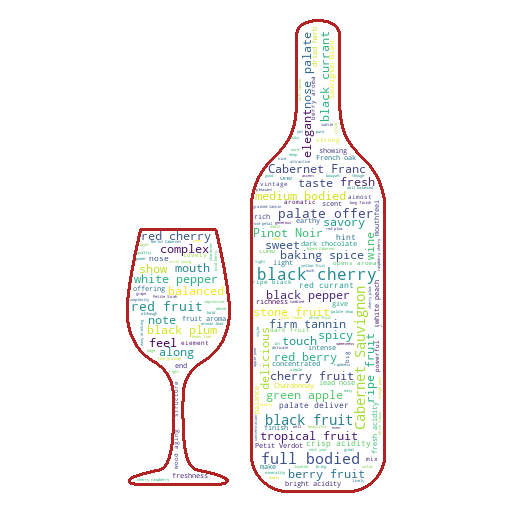
Voila! You created a word cloud in the shape of a wine bottle! It seems like wine descriptions most often mention black cherry, fruit flavors, and full-bodied characteristics of the wine. Now let's take a closer look at the reviews for each country and plot the word cloud using each country's flag. Below is an example that you will create soon:
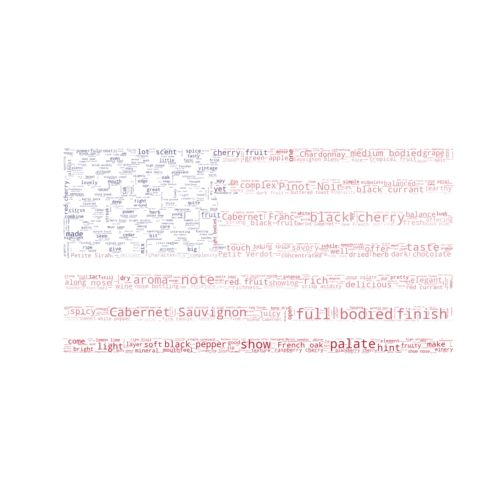
Creating a Word Cloud Following a Color Pattern
You can combine all the reviews of the five countries that have the most wines. To find those countries, you can either look at the plot country vs number of wines above or use the group that you got above to find the number of observations for each country (each group) and sort_values() with argument ascending=False to sort descending.
country.size().sort_values(ascending=False).head()
country
US          54504
France      22093
Italy       19540
Spain        6645
Portugal     5691
dtype: int64
So now you have 5 top countries: the US, France, Italy, Spain, and Portugal. You can change the number of countries by putting your chosen number insider head() like below
country.size().sort_values(ascending=False).head(10)
country
US           54504
France       22093
Italy        19540
Spain         6645
Portugal      5691
Chile         4472
Argentina     3800
Austria       3345
Australia     2329
Germany       2165
dtype: int64
For now, five countries should be enough.
To get all reviews for each country, you can concatenate all of the reviews using the " ".join(list) syntax, which joins all elements in a list, separating them by whitespace.
# Join all reviews of each country:
usa = " ".join(review for review in df[df["country"]=="US"].description)
fra = " ".join(review for review in df[df["country"]=="France"].description)
ita = " ".join(review for review in df[df["country"]=="Italy"].description)
spa = " ".join(review for review in df[df["country"]=="Spain"].description)
por = " ".join(review for review in df[df["country"]=="Portugal"].description)
Then, you can create the word cloud as outlined above. You can combine the two steps of creating and generating into one as below. The color mapping is done right before you plot the cloud using the ImageColorGenerator function from the WordCloud library.
# Generate a word cloud image
mask = np.array(Image.open("img/us.png"))
wordcloud_usa = WordCloud(stopwords=stopwords, background_color="white", mode="RGBA", max_words=1000, mask=mask).generate(usa)

# create coloring from image
image_colors = ImageColorGenerator(mask)
plt.figure(figsize=[7,7])
plt.imshow(wordcloud_usa.recolor(color_func=image_colors), interpolation="bilinear")
plt.axis("off")

# store to file
plt.savefig("img/us_wine.png", format="png")

plt.show()

Looks good! Now let's repeat with a review from France.
# Generate a word cloud image
mask = np.array(Image.open("img/france.png"))
wordcloud_fra = WordCloud(stopwords=stopwords, background_color="white", mode="RGBA", max_words=1000, mask=mask).generate(fra)

# create coloring from image
image_colors = ImageColorGenerator(mask)
plt.figure(figsize=[7,7])
plt.imshow(wordcloud_fra.recolor(color_func=image_colors), interpolation="bilinear")
plt.axis("off")

# store to file
plt.savefig("img/fra_wine.png", format="png")

#plt.show()
Please note that you should save the image after plotting to have the word cloud with the desired color pattern.

# Generate a word cloud image
mask = np.array(Image.open("img/italy.png"))
wordcloud_ita = WordCloud(stopwords=stopwords, background_color="white", max_words=1000, mask=mask).generate(ita)

# create coloring from image
image_colors = ImageColorGenerator(mask)
plt.figure(figsize=[7,7])
plt.imshow(wordcloud_ita.recolor(color_func=image_colors), interpolation="bilinear")
plt.axis("off")

# store to file
plt.savefig("img/ita_wine.png", format="png")

#plt.show()

Following Italy is Spain:
# Generate a word cloud image
mask = np.array(Image.open("img/spain.png"))
wordcloud_spa = WordCloud(stopwords=stopwords, background_color="white", max_words=1000, mask=mask).generate(spa)

# create coloring from image
image_colors = ImageColorGenerator(mask)
plt.figure(figsize=[7,7])
plt.imshow(wordcloud_spa.recolor(color_func=image_colors), interpolation="bilinear")
plt.axis("off")

# store to file
plt.savefig("img/spa_wine.png", format="png")
#plt.show()

Finally, Portugal:
# Generate a word cloud image
mask = np.array(Image.open("img/portugal.png"))
wordcloud_por = WordCloud(stopwords=stopwords, background_color="white", max_words=1000, mask=mask).generate(por)

# create coloring from image
image_colors = ImageColorGenerator(mask)
plt.figure(figsize=[7,7])
plt.imshow(wordcloud_por.recolor(color_func=image_colors), interpolation="bilinear")
plt.axis("off")

# store to file
plt.savefig("img/por_wine.png", format="png")
#plt.show()

The end result is in the below table to compare the masks and the word clouds. Which one is your favorite?


How to Interpret Word Clouds
So, we've now seen several word cloud examples and how to create them in Python. However, it's worth exploring how to interpret these data visualizations. Generally, the size of each word in the cloud represents its frequency or importance in the text. Typically, the more frequently a word appears in the text, the larger it will appear in the word cloud.
There are several things to bear in mind when interpreting word clouds:
- Pay attention to the size of the words: As mentioned, the size of each word in the cloud corresponds to its frequency or importance in the text. Therefore, larger words are generally more significant in the overall message of the text.
- Look for patterns: Are there any groups of words that appear together frequently? This can indicate a theme or topic that is important in the text.
- Consider the context: Remember that the word cloud only represents the words that appear in the text, and doesn't provide any information about their meaning or how they are being used. Therefore, it's important to think about the context of the text and the specific meanings of the words being used.
- Be wary of outliers: Sometimes, a word may appear very large in the word cloud simply because it appears frequently, even if it's not particularly meaningful or relevant to the overall message of the text. Keep an eye out for such outliers and try to focus on the words and patterns that are most significant.
Overall, a word cloud can be a useful tool for quickly visualizing the key themes and ideas in a text. However, it's important to keep in mind that it is just one tool among many for analyzing text data, and should be used in conjunction with other methods for deeper analysis and understanding.
Congratulations!
You made it! You have learned several ways to draw a word cloud in Python using the WordCloud library which would be helpful for the visualization of any text analysis. You also learn how to mask the cloud into any shape, using any color of your choice. If you want to practice your skills, consider the DataCamp's project: The Hottest Topics in Machine Learning
If you are interested in learning more about Natural Language Processing, take our Natural Language Processing Fundamentals in Python course.
