Course
Extreme Gradient Boosting with XGBoost
4 hr
60.7K
XGBoost is one of the most popular machine learning frameworks among data scientists. According to the Kaggle State of Data Science Survey 2021, almost 50% of respondents said they used XGBoost, ranking below only TensorFlow and Sklearn.
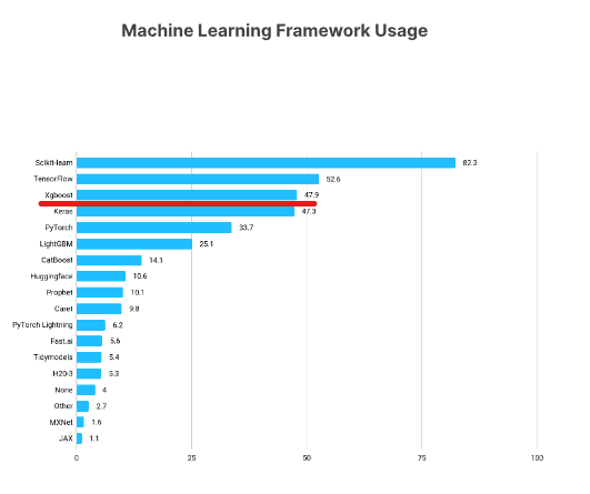
https://www.kaggle.com/kaggle-survey-2021
This XGBoost tutorial will introduce the key aspects of this popular Python framework, exploring how you can use it for your own machine learning projects.
Watch and learn more about using XGBoost in Python in this video from our course.
Throughout this tutorial, we will cover the key aspects of XGBoost, including:
Let’s get started!
Run and edit the code from this tutorial online
Run codeYou can install XGBoost like any other library through pip. This method of installation will also include support for your machine's NVIDIA GPU. If you want to install the CPU-only version, you can go with conda-forge:
$ pip install --user xgboost

# CPU only

$ conda install -c conda-forge py-xgboost-cpu

# Use NVIDIA GPU

$ conda install -c conda-forge py-xgboost-gpu
It’s recommended to install XGBoost in a virtual environment so as not to pollute your base environment.
We recommend running through the examples in the tutorial with a GPU-enabled machine. If you don’t have one, you can check out alternatives like DataLab or Google Colab.
If you decide to go with Colab, it has the old version of XGBoost installed, so you should call pip install --upgrade xgboost to get the latest version.
We will be working with the Diamonds dataset throughout the tutorial. It is built into the Seaborn library, or alternatively, you can also download it from Kaggle. It has a nice combination of numeric and categorical features and over 50k observations that we can comfortably showcase all the advantages of XGBoost.
import seaborn as sns

import pandas as pd

import numpy as np

import matplotlib.pyplot as plt

import warnings


warnings.filterwarnings("ignore")


diamonds = sns.load_dataset("diamonds")

diamonds.head()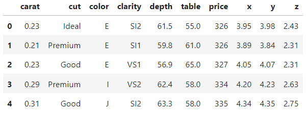
>>> diamonds.shape
(53940, 10)
In a typical real-world project, you would want to spend a lot more time exploring the dataset and visualizing its features. But since this data comes built-in to Seaborn, it is relatively clean.
So, we will just look at the 5-number summary of the numeric and categorical features and get going. You can spend a few moments to familiarize yourself with the dataset.
diamonds.describe()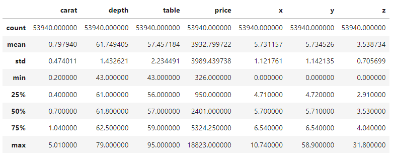
diamonds.describe(exclude=np.number)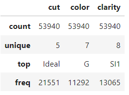
After you are done with exploration, the first step in any project is framing the machine learning problem and extracting the feature and target arrays based on the dataset.
In this tutorial, we will first try to predict diamond prices using their physical measurements, so our target will be the price column.
So, we are isolating the features into X and the target into y:
from sklearn.model_selection import train_test_split

# Extract feature and target arrays
X, y = diamonds.drop('price', axis=1), diamonds[['price']]
The dataset has three categorical columns. Normally, you would encode them with ordinal or one-hot encoding, but XGBoost has the ability to internally deal with categoricals.
The way to enable this feature is to cast the categorical columns into Pandas category data type (by default, they are treated as text columns):
# Extract text features
cats = X.select_dtypes(exclude=np.number).columns.tolist()

# Convert to Pandas category
for col in cats:
   X[col] = X[col].astype('category')
Now, when you print the dtypes attribute, you'll see that we have three category features:
>>> X.dtypes
carat       float64
cut        category
color      category
clarity    category
depth       float64
table       float64
x           float64
y           float64
z           float64
dtype: object
Let’s split the data into train, and test sets (0.25 test size):
# Split the data
X_train, X_test, y_train, y_test = train_test_split(X, y, random_state=1)
Now, the important part: XGBoost comes with its own class for storing datasets called DMatrix. It is a highly optimized class for memory and speed. That's why converting datasets into this format is a requirement for the native XGBoost API:
import xgboost as xgb

# Create regression matrices
dtrain_reg = xgb.DMatrix(X_train, y_train, enable_categorical=True)
dtest_reg = xgb.DMatrix(X_test, y_test, enable_categorical=True)
The class accepts both the training features and the labels. To enable automatic encoding of Pandas category columns, we also set enable_categorical to True.
Note:
Why are we going with the native API of XGBoost, rather than its Scikit-learn API? While it might be more comfortable to use the Sklearn API at first, later, you’ll realize that the native API of XGBoost contains some excellent features that the former doesn’t support. So, better get used to it from the beginning. However, there is a section at the end where we show how to switch between APIs in a single line of code even after you have trained models.
After building the DMatrices, you should choose a value for the objective parameter. It tells XGBoost the machine learning problem you are trying to solve and what metrics or loss functions to use to solve that problem.
For example, to predict diamond prices, which is a regression problem, you can use the common reg:squarederror objective. Usually, the name of the objective also contains the name of the loss function for the problem. For regression, it is common to use Root Mean Squared Error, which minimizes the square root of the squared sum of the differences between actual and predicted values. Here is how the metric would look like when implemented in NumPy:
import numpy as np

mse = np.mean((actual - predicted) ** 2)
rmse = np.sqrt(mse)
We’ll learn classification objectives later in the tutorial.
A note on the difference between a loss function and a performance metric: A loss function is used by machine learning models to minimize the differences between the actual (ground truth) values and model predictions. On the other hand, a metric (or metrics) is chosen by the machine learning engineer to measure the similarity between ground truth and model predictions.
In short, a loss function should be minimized while a metric should be maximized. A loss function is used during training to guide the model on where to improve. A metric is used during evaluation to measure overall performance.
The chosen objective function and any other hyperparameters of XGBoost should be specified in a dictionary, which by convention should be called params:
# Define hyperparameters
params = {"objective": "reg:squarederror", "tree_method": "gpu_hist"}
Inside this initial params, we are also setting tree_method to gpu_hist, which enables GPU acceleration. If you don't have a GPU, you can omit the parameter or set it to hist.
Now, we set another parameter called num_boost_round, which stands for number of boosting rounds. Internally, XGBoost minimizes the loss function RMSE in small incremental rounds (more on this later). This parameter specifies the amount of those rounds.
The ideal number of rounds is found through hyperparameter tuning. For now, we will just set it to 100:
# Define hyperparameters
params = {"objective": "reg:squarederror", "tree_method": "gpu_hist"}

n = 100
model = xgb.train(
   params=params,
   dtrain=dtrain_reg,
   num_boost_round=n,
)
When XGBoost runs on a GPU, it is blazing fast. If you didn’t receive any errors from the above code, the training was successful!
During the boosting rounds, the model object has learned all the patterns of the training set it possibly can. Now, we must measure its performance by testing it on unseen data. That's where our dtest_reg DMatrix comes into play:
from sklearn.metrics import mean_squared_error

preds = model.predict(dtest_reg)
This step of the process is called model evaluation (or inference). Once you generate predictions with predict, you pass them inside mean_squared_error function of Sklearn to compare against y_test:
rmse = mean_squared_error(y_test, preds, squared=False)

print(f"RMSE of the base model: {rmse:.3f}")
RMSE of the base model: 543.203
We’ve got a base score ~543$, which was the performance of a base model with default parameters. There are two ways we can improve it— by performing cross-validation and hyperparameter tuning. But before that, let’s see a quicker way of evaluating XGBoost models.
Training a machine learning model is like launching a rocket into space. You can control everything about the model up to the launch, but once it does, all you can do is stand by and wait for it to finish.
But the problem with our current training process is that we can’t even watch where the model is going. To solve this, we will use evaluation arrays that allow us to see model performance as it gets improved incrementally across boosting rounds.
First, let’s set up the parameters again:
params = {"objective": "reg:squarederror", "tree_method": "gpu_hist"}
n = 100
Next, we create a list of two tuples that each contain two elements. The first element is the array for the model to evaluate, and the second is the array’s name.
evals = [(dtrain_reg, "train"), (dtest_reg, "validation")]When we pass this array to the evals parameter of xgb.train, we will see the model performance after each boosting round:
evals = [(dtrain_reg, "train"), (dtest_reg, "validation")]

model = xgb.train(
   params=params,
   dtrain=dtrain_reg,
   num_boost_round=n,
   evals=evals,
)
You should get an output similar to the one below (shortened here to just 10 rows). You can see how the model minimizes the score from a whopping ~3931$ to just 543$.
What’s best is that we can see the model’s performance on both our training and validation sets. Usually, the training loss will be lower than validation since the model has already seen the former.
[0] train-rmse:3985.18329 validation-rmse:3930.52457
[1] train-rmse:2849.72257 validation-rmse:2813.20828
[2] train-rmse:2059.86648 validation-rmse:2036.66330
[3] train-rmse:1519.32314 validation-rmse:1510.02762
[4] train-rmse:1153.68171 validation-rmse:1153.91223
...
[95] train-rmse:381.93902 validation-rmse:543.56526
[96] train-rmse:380.97024 validation-rmse:543.51413
[97] train-rmse:380.75330 validation-rmse:543.36855
[98] train-rmse:379.65918 validation-rmse:543.42558
[99] train-rmse:378.30590 validation-rmse:543.20278
In real-world projects, you usually train for thousands of boosting rounds, which means that many rows of output. To reduce them, you can use the verbose_eval parameter, which forces XGBoost to print performance updates every vebose_eval rounds:
params = {"objective": "reg:squarederror", "tree_method": "gpu_hist"}
n = 100

evals = [(dtest_reg, "validation"), (dtrain_reg, "train")]


model = xgb.train(
   params=params,
   dtrain=dtrain_reg,
   num_boost_round=n,
   evals=evals,
   verbose_eval=10 # Every ten rounds
)

[OUT]:

[0] train-rmse:3985.18329 validation-rmse:3930.52457
[10] train-rmse:550.08330 validation-rmse:590.15023
[20] train-rmse:488.51248 validation-rmse:551.73431
[30] train-rmse:463.13288 validation-rmse:547.87843
[40] train-rmse:447.69788 validation-rmse:546.57096
[50] train-rmse:432.91655 validation-rmse:546.22557
[60] train-rmse:421.24046 validation-rmse:546.28601
[70] train-rmse:408.64125 validation-rmse:546.78238
[80] train-rmse:396.41125 validation-rmse:544.69846
[90] train-rmse:386.87996 validation-rmse:543.82192
[99] train-rmse:378.30590 validation-rmse:543.20278By now, you must have realized how important boosting rounds are. Generally, the more rounds there are, the more XGBoost tries to minimize the loss. But this doesn’t mean the loss will always go down. Let’s try with 5000 boosting rounds with the verbosity of 500:
params = {"objective": "reg:squarederror", "tree_method": "gpu_hist"}
n = 5000

evals = [(dtest_reg, "validation"), (dtrain_reg, "train")]


model = xgb.train(
   params=params,
   dtrain=dtrain_reg,
   num_boost_round=n,
   evals=evals,
   verbose_eval=250
)

[OUT]:

[0] train-rmse:3985.18329 validation-rmse:3930.52457
[500] train-rmse:195.89184 validation-rmse:555.90367
[1000] train-rmse:122.10746 validation-rmse:563.44888
[1500] train-rmse:84.18238 validation-rmse:567.16974
[2000] train-rmse:61.66682 validation-rmse:569.52584
[2500] train-rmse:46.34923 validation-rmse:571.07632
[3000] train-rmse:37.04591 validation-rmse:571.76912
[3500] train-rmse:29.43356 validation-rmse:572.43196
[4000] train-rmse:24.00607 validation-rmse:572.81287
[4500] train-rmse:20.45021 validation-rmse:572.89062
[4999] train-rmse:17.44305 validation-rmse:573.13200
We get the lowest loss before round 500. After that, even though training loss keeps going down, the validation loss (the one we care about) keeps increasing.
When given an unnecessary number of boosting rounds, XGBoost starts to overfit and memorize the dataset. This, in turn, leads to validation performance drop because the model is memorizing instead of generalizing.
Remember, we want the golden middle: a model that learned just enough patterns in training that it gives the highest performance on the validation set. So, how do we find the perfect number of boosting rounds, then?
We will use a technique called early stopping. Early stopping forces XGBoost to watch the validation loss, and if it stops improving for a specified number of rounds, it automatically stops training.
This means we can set as high a number of boosting rounds as long as we set a sensible number of early stopping rounds.
For example, let’s use 10000 boosting rounds and set the early_stopping_rounds parameter to 50. This way, XGBoost will automatically stop the training if validation loss doesn't improve for 50 consecutive rounds.
n = 10000


model = xgb.train(
   params=params,
   dtrain=dtrain_reg,
   num_boost_round=n,
   evals=evals,
   verbose_eval=50,
   # Activate early stopping
   early_stopping_rounds=50
)

[OUT]:

[0] train-rmse:3985.18329 validation-rmse:3930.52457
[50] train-rmse:432.91655 validation-rmse:546.22557
[100] train-rmse:377.66173 validation-rmse:542.92457
[150] train-rmse:334.27548 validation-rmse:542.79733
[167] train-rmse:321.04059 validation-rmse:543.35679
As you can see, the training stopped after the 167th round because the loss stopped improving for 50 rounds before that.
At the beginning of the tutorial, we set aside 25% of the dataset for testing. The test set would allow us to simulate the conditions of a model in production, where it must generate predictions for unseen data.
But only a single test set would not be enough to measure how a model would perform in production accurately. For example, if we perform hyperparameter tuning using only a single training and a single test set, knowledge about the test set would still “leak out.” How?
Since we try to find the best value of a hyperparameter by comparing the validation performance of the model on the test set, we will end up with a model that is configured to perform well only on that particular test set. Instead, we want a model that performs well across the board — on any test set we throw at it.
A possible workaround is splitting the data into three sets. The model trains on the first set, the second set is used for evaluation and hyperparameter tuning, and the third is the final one we test the model before production.
But when data is limited, splitting data into three sets will make the training set sparse, which hurts model performance.
The solution to all these problems is cross-validation. In cross-validation, we still have two sets: training and testing.
While the test set waits in the corner, we split the training into 3, 5, 7, or k splits or folds. Then, we train the model k times. Each time, we use k-1 parts for training and the final kth part for validation. This process is called k-fold cross-validation:
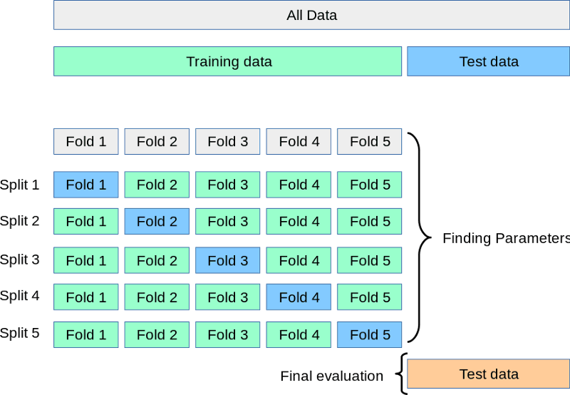
Source: https://scikit-learn.org/stable/modules/cross_validation.html
Above is a visual depiction of a 5-fold cross-validation. After all folds are done, we can take the mean of the scores as the final, most realistic performance of the model.
Let’s perform this process in code using the cv function of XGB:
params = {"objective": "reg:squarederror", "tree_method": "gpu_hist"}
n = 1000

results = xgb.cv(
   params, dtrain_reg,
   num_boost_round=n,
   nfold=5,
   early_stopping_rounds=20
)
The only difference with the train function is adding the nfold parameter to specify the number of splits. The results object is now a DataFrame containing each fold's results:
results.head()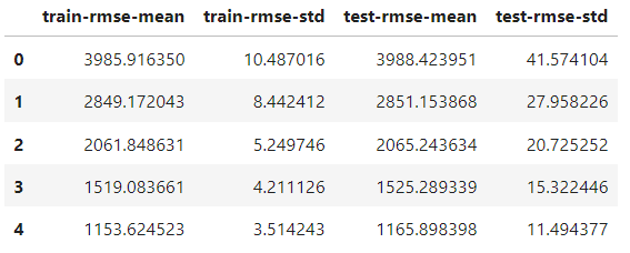
It has the same number of rows as the number of boosting rounds. Each row is the average of all splits for that round. So, to find the best score, we take the minimum of the test-rmse-mean column:
best_rmse = results['test-rmse-mean'].min()

best_rmse
550.8959336674216
Note that this method of cross-validation is used to see the true performance of the model. Once satisfied with its score, you must retrain it on the full data before deployment.
Building an XGBoost classifier is as easy as changing the objective function; the rest can stay the same.
The two most popular classification objectives are:
binary:logistic - binary classification (the target contains only two classes, i.e., cat or dog)multi:softprob - multi-class classification (more than two classes in the target, i.e., apple/orange/banana)Performing binary and multi-class classification in XGBoost is almost identical, so we will go with the latter. Let’s prepare the data for the task first.
We want to predict the cut quality of diamonds given their price and their physical measurements. So, we will build the feature/target arrays accordingly:
from sklearn.preprocessing import OrdinalEncoder

X, y = diamonds.drop("cut", axis=1), diamonds[['cut']]

# Encode y to numeric
y_encoded = OrdinalEncoder().fit_transform(y)

# Extract text features
cats = X.select_dtypes(exclude=np.number).columns.tolist()

# Convert to pd.Categorical
for col in cats:
   X[col] = X[col].astype('category')

# Split the data
X_train, X_test, y_train, y_test = train_test_split(X, y_encoded, random_state=1, stratify=y_encoded)
The only difference is that since XGBoost only accepts numbers in the target, we are encoding the text classes in the target with OrdinalEncoder of Sklearn.
Now, we build the DMatrices…
# Create classification matrices
dtrain_clf = xgb.DMatrix(X_train, y_train, enable_categorical=True)
dtest_clf = xgb.DMatrix(X_test, y_test, enable_categorical=True)
…and set the objective to multi:softprob. This objective also requires the number of classes to be set by us:
params = {"objective": "multi:softprob", "tree_method": "gpu_hist", "num_class": 5}
n = 1000

results = xgb.cv(
   params, dtrain_clf,
   num_boost_round=n,
   nfold=5,
   metrics=["mlogloss", "auc", "merror"],
)
During cross-validation, we are asking XGBoost to watch three classification metrics which report model performance from three different angles. Here is the result:
results.keys()

Index(['train-mlogloss-mean', 'train-mlogloss-std', 'train-auc-mean',

      'train-auc-std', 'train-merror-mean', 'train-merror-std',

      'test-mlogloss-mean', 'test-mlogloss-std', 'test-auc-mean',

      'test-auc-std', 'test-merror-mean', 'test-merror-std'],

     dtype='object')
To see the best AUC score, we take the maximum of test-auc-mean column:
>>> results['test-auc-mean'].max()
0.9402233623451636
Even the default configuration gave us 94% performance, which is great.
So far, we have been using the native XGBoost API, but its Sklearn API is pretty popular as well.
Sklearn is a vast framework with many machine learning algorithms and utilities and has an API syntax loved by almost everyone. Therefore, XGBoost also offers XGBClassifier and XGBRegressor classes so that they can be integrated into the Sklearn ecosystem (at the loss of some of the functionality).
If you want to only use the Scikit-learn API whenever possible and only switch to native when you need access to extra functionality, there is a way.
After training the XGBoost classifier or regressor, you can convert it using the get_booster method:
import xgboost as xgb

# Train a model using the scikit-learn API
xgb_classifier = xgb.XGBClassifier(n_estimators=100, objective='binary:logistic', tree_method='hist', eta=0.1, max_depth=3, enable_categorical=True)
xgb_classifier.fit(X_train, y_train)

# Convert the model to a native API model
model = xgb_classifier.get_booster()
The model object will behave in the exact same way we've seen throughout this tutorial.
We’ve covered a lot of important topics in this XGBoost tutorial, but there are still so many things to learn.
You can check out the XGBoost parameters page, which teaches you how to configure the parameters to squeeze out every last performance from your models.
If you are looking for a comprehensive, all-in-one resource to learn the library, check out our Extreme Gradient Boosting With XGBoost course.
Learn more about Python and XGBoost
Course
Course
Course
Tutorial
Bex Tuychiev
Tutorial
Oluseye Jeremiah
Tutorial
Kurtis Pykes
Tutorial
Avinash Navlani
Tutorial
Matthew Przybyla
Tutorial
Avinash Navlani