Let's say the target is monthly electricity demand. Models like ARIMA and SARIMA only look at the past values of the series and their own past forecast errors. But demand also depends on outside factors like temperature: a hot summer increases it, and so does a cold winter. If the model can't see these factors, it treats every unusual month as noise and makes the same mistake the next time the weather changes.
SARIMAX solves this problem by adding external, or exogenous, variables on top of a seasonal ARIMA model. It still learns trend and seasonality from the history of the series, but it also uses outside information that explains what the past values can't.
If you need a starter in manipulating, interpreting, and visualizing time series data in Python, enroll in our Time Series in Python track to dial in the fundamentals in a week.
What Is SARIMAX?
SARIMAX is a seasonal ARIMA model that can also use external predictors. Specifically, the name stands for Seasonal AutoRegressive Integrated Moving Average with eXogenous regressors.
SARIMAX works by predicting a target series from four sources of information:
- Past values: Demand in the most recent months
- Past forecast errors: How far off the model was in the most recent months
- Seasonal patterns: Demand in the same month of previous years
- Exogenous variables: Outside data you add to the model, such as average monthly temperature
Let's say the goal is to forecast electricity demand for next July. SARIMAX looks at demand in the past couple of months, at demand in previous Julys, and at the expected temperature for July. The first two are inside the series and the temperature comes from outside.
You write the model as SARIMAX(p, d, q)(P, D, Q, S). The first set of parameters covers short-term behavior, and the second set covers the seasonal component, where S is the number of time steps in one cycle. For monthly data with a yearly pattern, S is 12.
The exogenous variables are not included in this notation. You pass them to the model separately, as their own input.
How SARIMAX Works
SARIMAX has two groups of terms, and the exogenous variables go on top of them.
The nonseasonal terms (p, d, q) model short-term behavior:
-
Autoregressive order
p: How many past values the model uses. Withp = 2, demand this month depends on demand in the previous two months -
Differencing order
d: How many times the model differences the series to remove a trend. Withd = 1, the model works with month-over-month changes instead of raw demand -
Moving average order
q: How many past forecast errors the model uses. If the model underestimated demand last month, that error goes into this month's prediction
The seasonal terms (P, D, Q, S) do the same thing, but at seasonal lags:
-
Seasonal autoregressive order
P: How many past seasons the model looks at. WithP = 1and monthly data, demand this July depends on demand last July -
Seasonal differencing order
D: How many times the model differences the series at the seasonal lag. WithD = 1, the model compares this July to last July, which removes the repeating yearly pattern -
Seasonal moving average order
Q: How many past forecast errors at seasonal lags the model uses, such as the error from last July -
Seasonal period
S: How many time steps one cycle has. It's 12 for monthly data with a yearly pattern and 7 for daily data with a weekly pattern
Exogenous variables add information the series doesn't have.
In the electricity demand example, that's temperature. A hot summer or a cold winter increases demand, and past demand values can't tell the model what next month's weather will be. The month-of-year pattern already comes from the seasonal terms, so temperature is the only external variable the example needs.
In statsmodels, SARIMAX is a linear regression on the exogenous variables, where the errors follow a seasonal ARIMA process. With one exogenous variable, it looks like this:
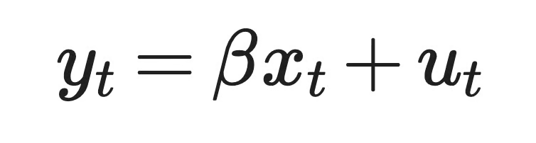
SARIMAX with one exogenous variable
Here, y_t is electricity demand in month t, x_t is the temperature in that month, beta is the temperature coefficient, and u_t is the part of demand temperature doesn't explain. The nonseasonal and seasonal terms model u_t.
In plain English, that's temperature explaining part of the demand, and the SARIMA terms modeling everything else.
Here's a more visual overview:
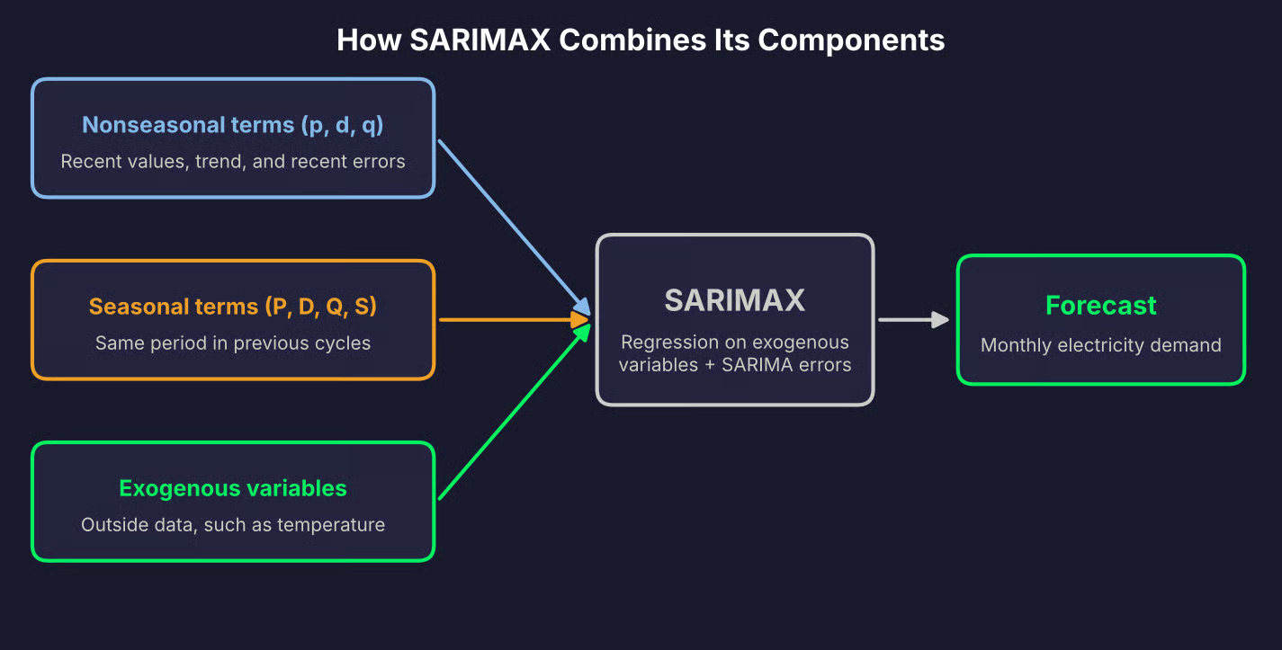
SARIMAX components
ARIMA vs. SARIMA vs. ARIMAX vs. SARIMAX
These four models belong to the same family. The differences are subtle, but you'll understand them after one reading.
ARIMA models a series from its own past values and past forecast errors. SARIMA adds seasonal terms on top of that, so it can model patterns that repeat every S time steps. ARIMAX adds exogenous variables to ARIMA, but it doesn't have seasonal terms by default. SARIMAX has both.
That's why SARIMAX can represent the other models as special cases. If you don't pass any exogenous variables, you get a SARIMA model. If you set all seasonal orders to zero, you get a nonseasonal ARIMAX model. And with neither, it's an ARIMA model.
But unfortunately, the terminology isn't consistent across packages.
The textbook ARIMAX puts exogenous variables directly into the ARIMA equation, next to the past values of the series. statsmodels' SARIMAX fits a regression with SARIMA errors instead, as shown in the previous section. The two forms estimate different coefficients, so the same temperature variable can get a different coefficient depending on the package.
Class and function names don't match either. The ARIMA class in statsmodels also accepts seasonal terms and exogenous variables. In R, the forecast package handles external regressors through the xreg argument of Arima() and auto.arima(). So because of that, remember to check how each package defines the model before you compare results across tools.
Here's a quick recap:
| Seasonality? | External variables? | |
|---|---|---|
| ARIMA | No | No |
| SARIMA | Yes | No |
| ARIMAX | Not by default | Yes |
| SARIMAX | Yes | Yes |
ARIMA model family comparison
When to Use SARIMAX
SARIMAX makes sense when the target has a recurring seasonal pattern and outside variables can improve the forecast.
For example:
- Electricity demand: Temperature and calendar effects such as public holidays, on top of the yearly cycle
- Retail sales: Promotions, prices, and holiday periods
- Hotel bookings: Local events and room prices, on top of the yearly travel season
- Public transport ridership: Weather and school holidays, on top of a weekly pattern in daily data
But SARIMAX isn't always the right choice. A simpler model can do the same job in these two cases:
- No meaningful seasonality: If the series doesn't repeat a pattern, seasonal terms only add parameters to estimate. ARIMA or ARIMAX is enough
- Predictors don't improve accuracy: If exogenous variables don't reduce the error on a held-out test period, remove them and use SARIMA. A better fit on the training data doesn't count
The thing to remember here is that SARIMAX needs values for every exogenous variable in the forecast period.
Some values are known in advance, for example, public holidays or planned promotions. Others, such as temperature, have to be forecast separately before SARIMAX can use them. If you can't get future values for a predictor, you can't use it in the forecast.
How to Build a SARIMAX Model in Python
In this section, I'll build a SARIMAX model with statsmodels, from raw data to a 12-month forecast.
The example uses synthetic monthly electricity demand with temperature as the outside variable. It's small and reproducible, and it follows the same story as the rest of the article.
Prepare the data
The dataset covers ten years of monthly data, from January 2015 to December 2024.
Demand has an upward trend, a yearly calendar pattern that changes slowly over time, a weather effect, and noise. Two temperature readings are missing on purpose, so you can see how to work with gaps:
import numpy as np
import pandas as pd
import matplotlib.pyplot as plt
import warnings

warnings.filterwarnings("ignore")

rng = np.random.default_rng(10)

# Monthly timestamps from January 2015 to December 2024
dates = pd.date_range(start="2015-01-01", periods=120, freq="MS")
month = dates.month.to_numpy()

# Average monthly temperature in degrees Celsius
temperature = 12 + 11 * np.sin(2 * np.pi * (month - 4) / 12) + rng.normal(0, 2, 120)

# Calendar pattern that repeats every year and changes slowly over time
calendar_effect = 15 * np.cos(2 * np.pi * (month - 1) / 12)
for t in range(12, 120):
    calendar_effect[t] = calendar_effect[t - 12] + rng.normal(0, 2.5)

# Short-term noise where each month carries over part of the previous one
noise = np.zeros(120)
for t in range(1, 120):
    noise[t] = 0.5 * noise[t - 1] + rng.normal(0, 6)

# Demand in GWh: upward trend, calendar pattern, weather effect, and noise
trend = np.linspace(500, 560, 120)
heating_demand = 6 * np.clip(18 - temperature, 0, None)
cooling_demand = 9 * np.clip(temperature - 18, 0, None)
demand = trend + calendar_effect + heating_demand + cooling_demand + noise

df = pd.DataFrame(
    {"demand_gwh": demand.round(1), "temperature": temperature.round(1)},
    index=dates,
)

# Two missing temperature readings
df.loc[["2018-07-01", "2021-02-01"], "temperature"] = np.nan

print(df.head())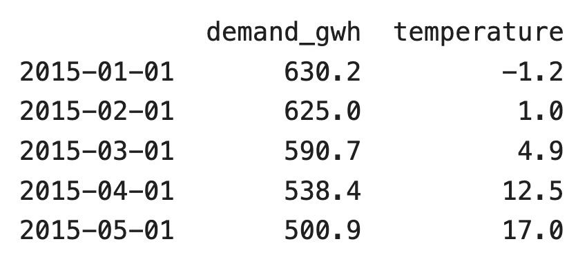
The first five rows of the dataset
Or, if you prefer a visual overview:
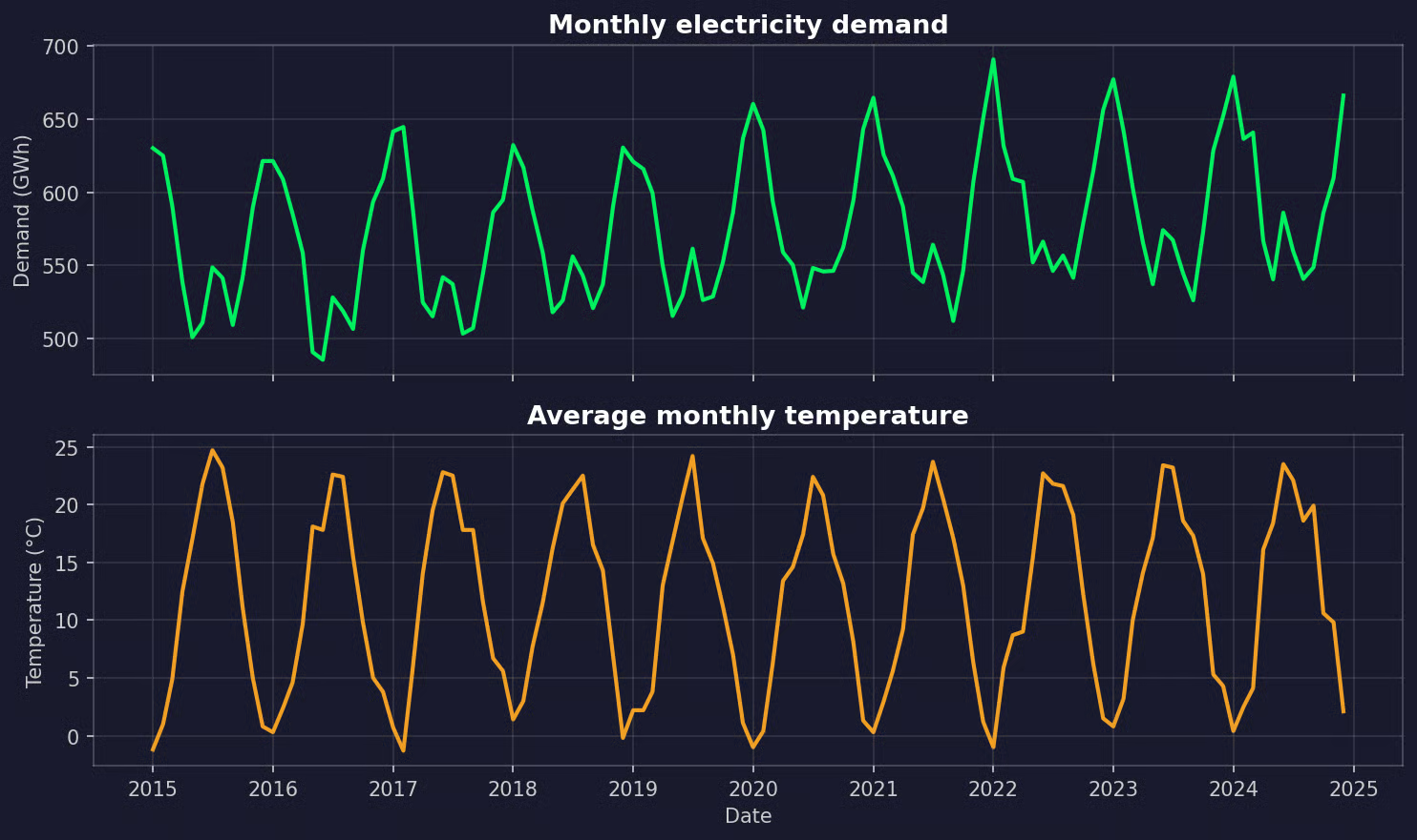
The temperature dataset
If you're working with your own data, load it with pd.read_csv() and set the date column as the index. The rest of the workflow stays the same.
SARIMAX needs a time index with a consistent frequency. The .asfreq() method sets it to monthly and inserts an empty row for any missing month. Then you can count the gaps and fill them:
df = df.asfreq("MS")
print(df.isna().sum())

df["temperature"] = df["temperature"].interpolate()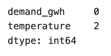
Interpolating temperature gaps
Linear interpolation works here because temperature changes smoothly from month to month. Don't do the same for the target if large chunks of it are missing. You'd be teaching the model on made-up values.
Next, the exogenous variables. Demand goes up when it's cold and when it's hot, but a straight-line regression on raw temperature can't model a U-shape. So I'll split temperature into two features:
- Heating degrees: How many degrees the average temperature is below 18 degrees Celsius, and zero otherwise
- Cooling degrees: How many degrees the average temperature is above 18 degrees Celsius, and zero otherwise
df["heating_degrees"] = (18 - df["temperature"]).clip(lower=0)
df["cooling_degrees"] = (df["temperature"] - 18).clip(lower=0)
Now split the data into the target y and the exogenous variables X. The split has to be chronological: the model trains on the past and gets tested on the future. A random split would leak future information into training:
y = df["demand_gwh"]
X = df[["heating_degrees", "cooling_degrees"]]

y_train, y_test = y[:"2022-12"], y["2023-01":]
X_train, X_test = X[:"2022-12"], X["2023-01":]

print(f"Train: {len(y_train)} months, Test: {len(y_test)} months")
Train/test split
The thing to remember here is that X_test has actual observed temperatures. In a real forecast, you wouldn't know them in advance - you'd have a weather forecast at best. This means the test score you'll see later is optimistic. Use observed predictor values for evaluation only if the same values would be available at forecast time, like public holidays or planned prices.
Explore seasonality and stationarity
Start with a plot. You're looking for trends, seasonal cycles, and sudden changes:
from statsmodels.tsa.seasonal import seasonal_decompose

fig, ax = plt.subplots(figsize=(10, 4))
y_train.plot(ax=ax, title="Monthly electricity demand (GWh)")
plt.show()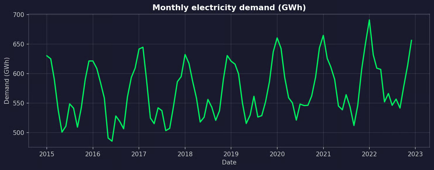
Monthly electricity demand in the training period
Demand goes up over time, and it peaks every winter with a smaller peak every summer. The pattern repeats every 12 months.
A seasonal decomposition will split the series into trend, seasonal, and residual components, so you can confirm the seasonal period S:
decomposition = seasonal_decompose(y_train, model="additive", period=12)
decomposition.plot()
plt.show()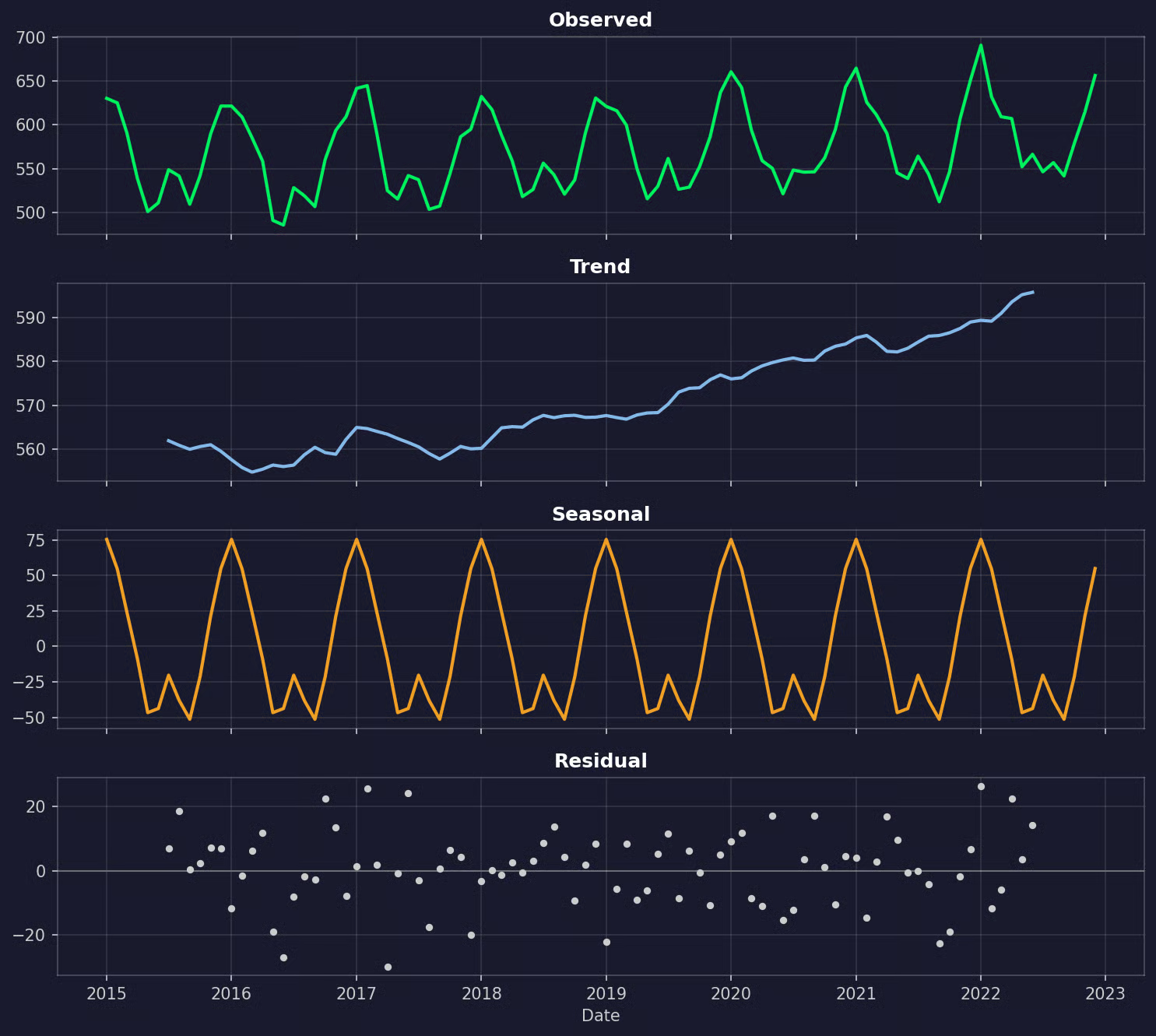
Seasonal decomposition of electricity demand
The seasonal component repeats every year, so S = 12.
ARIMA-family models need a stationary series - one whose mean and variance don't change over time. Demand isn't stationary because it has a trend and a seasonal cycle.
Differencing is a way to get around that:
-
Regular differencing (
d): Subtracts last month's value from this month's value. It removes a trend -
Seasonal differencing (
D): Subtracts the value from the same month last year. It removes a repeating seasonal pattern, and it also removes a linear trend
The Augmented Dickey-Fuller (ADF) test checks for stationarity. Its null hypothesis is that the series isn't stationary, so a small p-value (below 0.05) is evidence that it is:
from statsmodels.tsa.stattools import adfuller

series_versions = {
    "Original": y_train,
    "Seasonally differenced (D=1)": y_train.diff(12).dropna(),
    "Both differences (d=1, D=1)": y_train.diff().diff(12).dropna(),
}

for name, series in series_versions.items():
    adf_stat, p_value = adfuller(series)[:2]
    print(f"{name}: ADF statistic = {adf_stat:.2f}, p-value = {p_value:.4f}")
ADF test result
The original series isn't stationary. Seasonal differencing alone fixes it, so regular differencing on top adds nothing. Use the smallest amount of differencing that works - extra differences add noise to the series and make the model harder to fit.
So the choice is d = 0 and D = 1.
But treat the ADF test as supporting evidence only. It tells you nothing about p, q, P, or Q, and with short series it can give different answers depending on its settings.
Select candidate parameters
ACF and PACF plots help you choose candidate values for the remaining orders:
-
ACF (autocorrelation function): Shows the correlation between the series and its own lagged values. Spikes in the ACF point to moving average terms,
qat short lags andQat seasonal lags -
PACF (partial autocorrelation function): Shows the same correlation, but removes the effect of the lags in between. Spikes in the PACF point to autoregressive terms,
pat short lags andPat seasonal lags
You should plot both for the seasonally differenced series, since that's the series the model works with:
from statsmodels.graphics.tsaplots import plot_acf, plot_pacf

y_seasonal_diff = y_train.diff(12).dropna()

fig, axes = plt.subplots(1, 2, figsize=(12, 4))
plot_acf(y_seasonal_diff, lags=24, ax=axes[0])
plot_pacf(y_seasonal_diff, lags=24, ax=axes[1])
plt.show()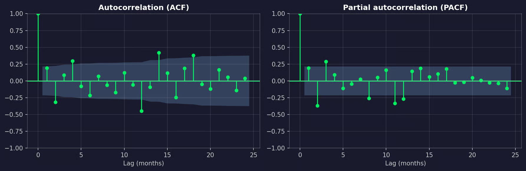
ACF and PACF plots of seasonally differenced electricity demand
The ACF has a clear negative spike at lag 12 and nothing at lag 24. That's the typical sign of a seasonal moving average term, so Q = 1 is a good candidate. Both plots also show a couple of spikes at short lags, so p and q are worth testing.
The next step is to fit a small set of candidate models and compare them with AIC or BIC. Both score how well a model fits the training data and penalize extra parameters. Lower is better, and BIC penalizes complexity more than AIC does:
import itertools
from statsmodels.tsa.statespace.sarimax import SARIMAX

candidates = []
for p, q, P, Q in itertools.product([0, 1], [0, 1], [0, 1], [0, 1]):
    candidate = SARIMAX(
        y_train,
        exog=X_train,
        order=(p, 0, q),
        seasonal_order=(P, 1, Q, 12),
        trend="c",
    ).fit(disp=False)
    candidates.append({
        "order": (p, 0, q),
        "seasonal_order": (P, 1, Q, 12),
        "AIC": round(candidate.aic, 1),
        "BIC": round(candidate.bic, 1),
    })

print(pd.DataFrame(candidates).sort_values("AIC").head(5).to_string(index=False))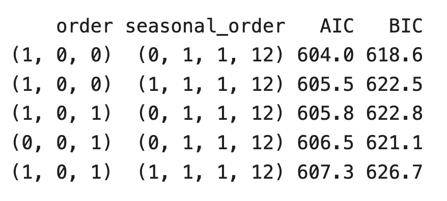
AIC and BIC results
SARIMAX(1, 0, 0)(0, 1, 1, 12) wins on both AIC and BIC. It's also one of the simplest models in the list.
The trend="c" argument adds a constant. With seasonal differencing, a constant models the year-over-year increase in demand.
You'll find tools like auto_arima() from the pmdarima library that run this search for you. They're handy for a first pass, but AIC and BIC only measure fit on the training data. Before you trust a model, test it on data it hasn't seen.
Fit the model
Pass the target as the first argument and the exogenous variables through exog. The order argument takes (p, d, q), and seasonal_order takes (P, D, Q, S):
model = SARIMAX(
    y_train,
    exog=X_train,
    order=(1, 0, 0),
    seasonal_order=(0, 1, 1, 12),
    trend="c",
)
results = model.fit(disp=False)
print(results.summary())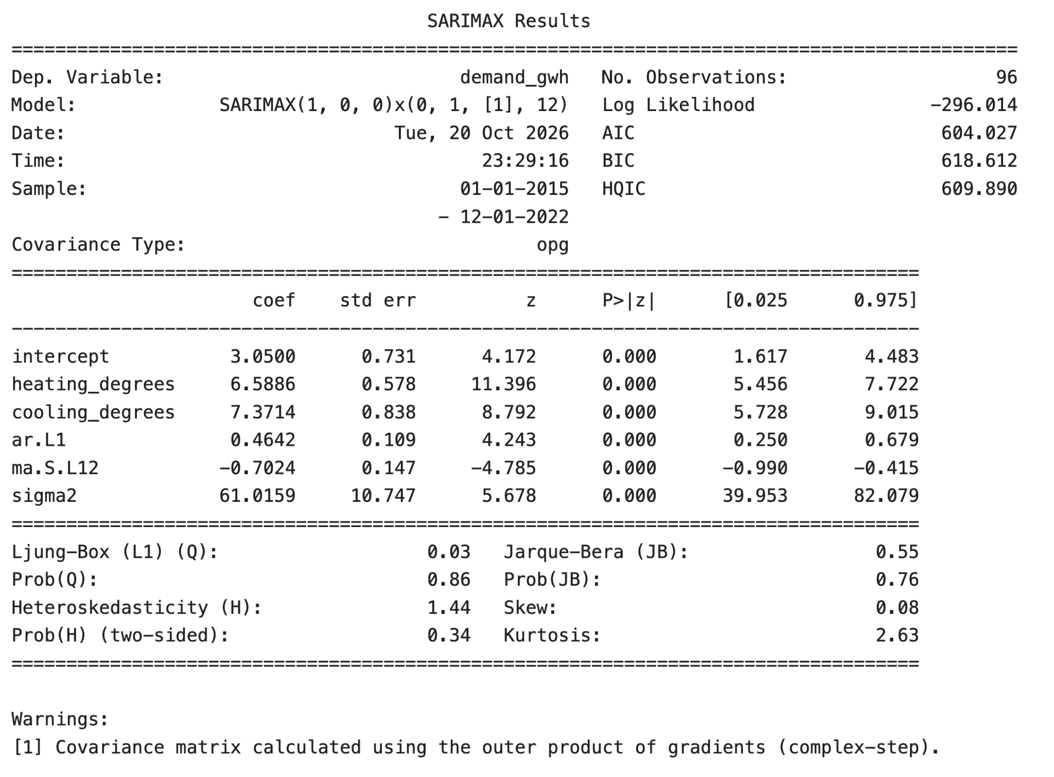
SARIMAX model summary
Here's how to read the coefficient table:
-
heating_degrees: Each extra heating degree goes with about 6.6 GWh of extra demand, with everything else in the model fixed -
cooling_degrees: Each extra cooling degree goes with about 7.4 GWh of extra demand -
ar.L1: About 46% of last month's unexplained difference carries over into this month -
ma.S.L12: The seasonal moving average term, which corrects the forecast based on the error from the same month last year -
sigma2: The variance of the remaining noise
All coefficients have p-values close to zero, so each term adds something to the model.
But these coefficients describe relationships inside the fitted model, not causes. Here, I generated the data with temperature as a cause of demand, so the reading is safe. In real data, a predictor can look important because it moves together with something the model doesn't see.
Diagnose and evaluate the model
A good model leaves behind residuals that look like random noise. If the residuals still have a pattern, the model has missed something.
The .plot_diagnostics() method gives you four plots in one call:
from statsmodels.stats.diagnostic import acorr_ljungbox

results.plot_diagnostics(figsize=(12, 8))
plt.show()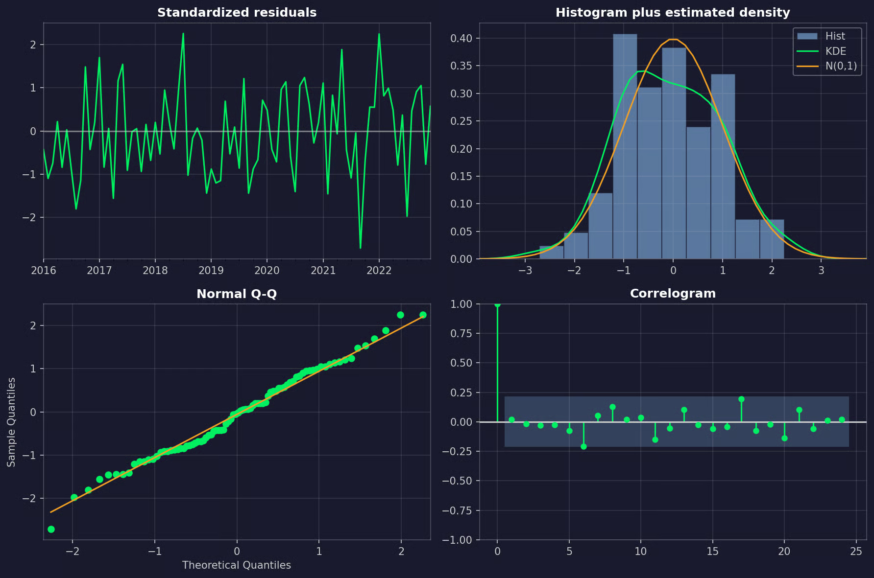
Residual diagnostics plot
Here's what to look for:
- Standardized residuals: No trend, no repeating pattern, and no stretches where the spread gets much wider
- Histogram and Q-Q plot: Points close to a normal distribution
- Correlogram: No spikes outside the confidence band, especially at lag 12 - a spike there means the model hasn't fully handled the seasonality
The Ljung-Box test gives you the same check as a number. Its null hypothesis is that the residuals have no autocorrelation up to a given lag, so you want large p-values:
# Skip the first 13 residuals, which come from the differencing start-up period
print(acorr_ljungbox(results.resid[13:], lags=[12, 24]))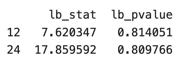
The Ljung-Box test results
Both p-values are well above 0.05, so the residuals look like noise.
Now for the part that matters most - accuracy on data the model hasn't seen. The .get_forecast() method predicts the 24 test months, and it needs the exogenous values for those months.
A forecast number means little on its own, so I'll compare SARIMAX against two baselines:
- Seasonal naive forecast: Repeats the values from the last 12 months of training data
- SARIMA: The same model, but without the exogenous variables
from sklearn.metrics import mean_absolute_error, root_mean_squared_error

sarimax_pred = results.get_forecast(steps=len(y_test), exog=X_test).predicted_mean

# Baseline 1: repeat the last 12 observed months
naive_pred = pd.Series(np.tile(y_train[-12:].to_numpy(), 2), index=y_test.index)

# Baseline 2: the same model without exogenous variables
sarima_results = SARIMAX(
    y_train, order=(1, 0, 0), seasonal_order=(0, 1, 1, 12), trend="c"
).fit(disp=False)
sarima_pred = sarima_results.get_forecast(steps=len(y_test)).predicted_mean

for name, pred in [("SARIMAX", sarimax_pred), ("SARIMA", sarima_pred), ("Seasonal naive", naive_pred)]:
    mae = mean_absolute_error(y_test, pred)
    rmse = root_mean_squared_error(y_test, pred)
    print(f"{name:<15} MAE = {mae:.2f} GWh, RMSE = {rmse:.2f} GWh")

fig, ax = plt.subplots(figsize=(10, 4))
y_train["2020":].plot(ax=ax, label="Train")
y_test.plot(ax=ax, label="Test")
sarimax_pred.plot(ax=ax, label="SARIMAX", linestyle="--")
naive_pred.plot(ax=ax, label="Seasonal naive", linestyle=":")
ax.legend()
plt.show()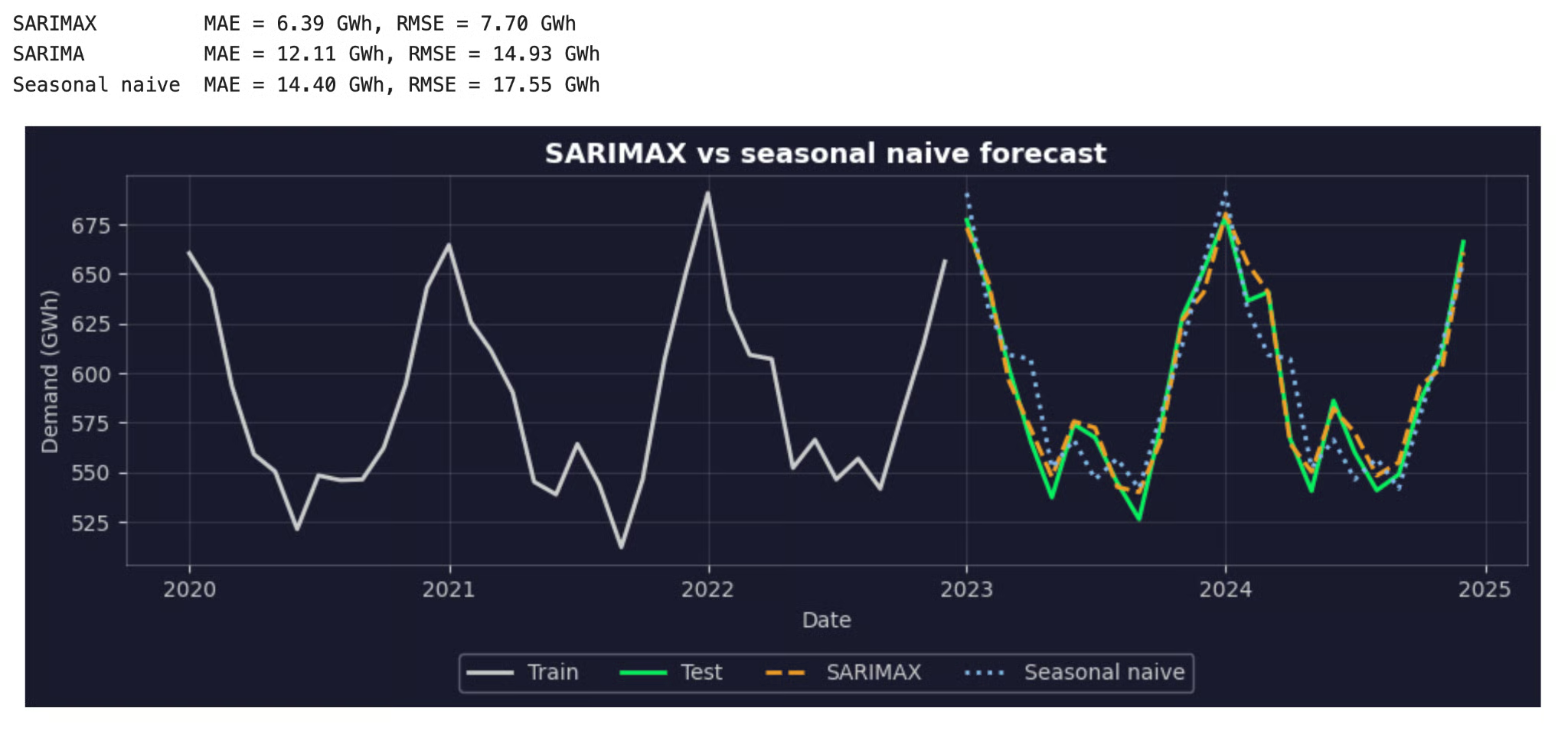
SARIMAX and seasonal naive forecasts versus actual demand in the test set
MAE (mean absolute error) is the average size of the error in GWh. RMSE (root mean squared error) punishes large errors more.
SARIMAX has about half the error of SARIMA on both metrics. The seasonal terms alone can't predict an unusually cold January or a hot July, and the temperature features can.
Remember, this result uses observed test-period temperatures. With weather forecasts in their place, the gap would be smaller.
Forecast future values
Once you're happy with the model, refit it on all the data, so the forecast starts from the most recent month.
Then forecast with .get_forecast(). You need a value for every exogenous variable in every future month. If one is missing, statsmodels raises an error.
Where those values come from depends on the variable. For example:
- Known calendar features: Holidays and the number of working days are known years ahead
- Planned business decisions: Prices and promotions are known if your team has already scheduled them
- Weather: Temperature needs a separate forecast, from a weather service or from another model
- Historical averages: If you have nothing better, use the average value for each calendar month from past data
I'll use the last option here as a stand-in for a weather forecast:
final_results = SARIMAX(
    y, exog=X, order=(1, 0, 0), seasonal_order=(0, 1, 1, 12), trend="c"
).fit(disp=False)

future_dates = pd.date_range(start="2025-01-01", periods=12, freq="MS")

# Stand-in for a weather forecast: the average temperature of each calendar month
monthly_normals = df.groupby(df.index.month)["temperature"].mean()
future_temperature = monthly_normals.loc[future_dates.month].to_numpy()

X_future = pd.DataFrame({
    "heating_degrees": np.clip(18 - future_temperature, 0, None),
    "cooling_degrees": np.clip(future_temperature - 18, 0, None),
}, index=future_dates)

forecast = final_results.get_forecast(steps=12, exog=X_future)
forecast_df = pd.concat([forecast.predicted_mean.rename("forecast"), forecast.conf_int(alpha=0.05)], axis=1)
print(forecast_df.round(1))

fig, ax = plt.subplots(figsize=(10, 4))
y["2021":].plot(ax=ax, label="Observed")
forecast.predicted_mean.plot(ax=ax, label="Forecast")
ci = forecast.conf_int(alpha=0.05)
ax.fill_between(ci.index, ci.iloc[:, 0], ci.iloc[:, 1], alpha=0.3, label="95% interval")
ax.legend()
plt.show()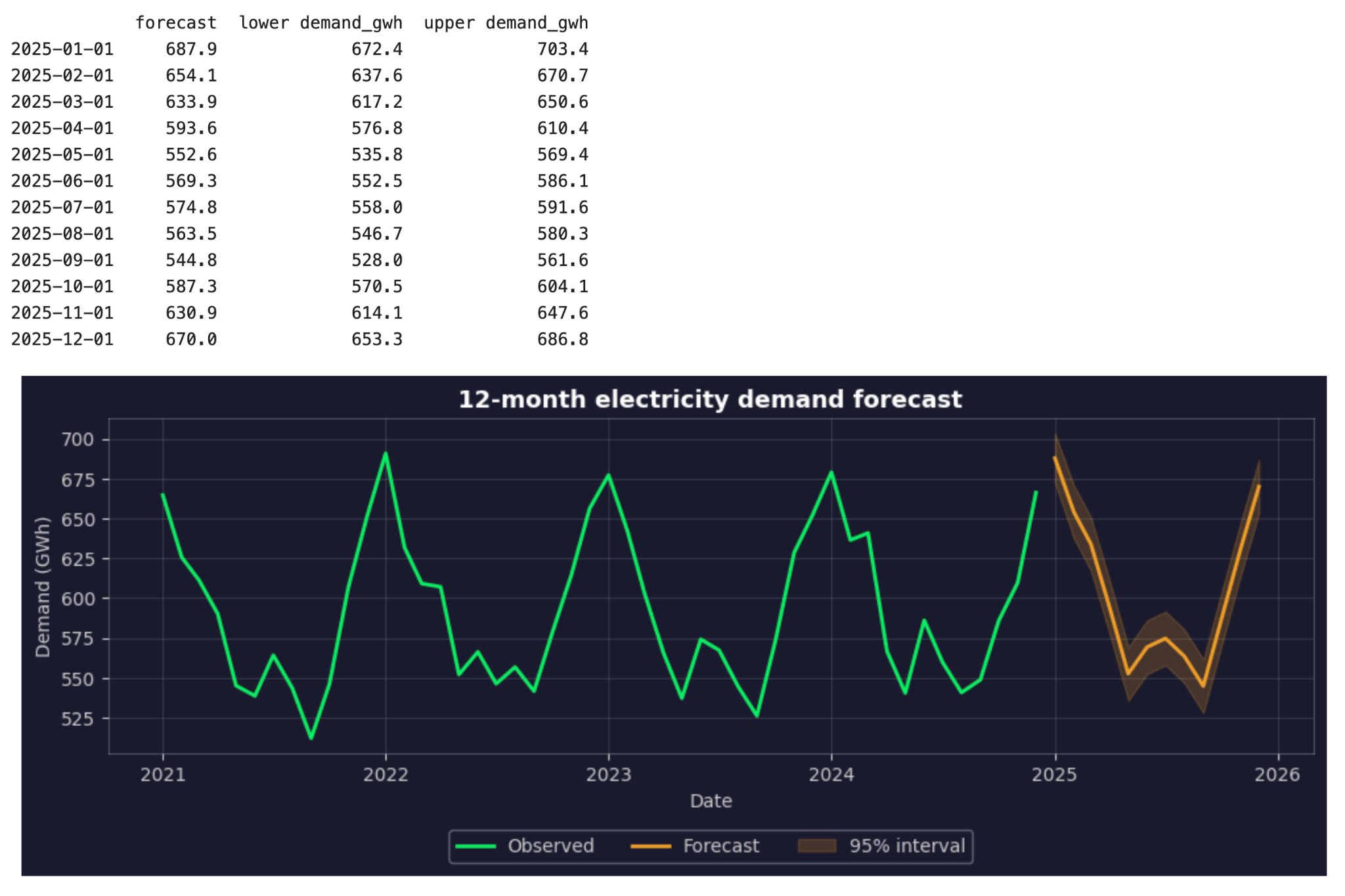
12-month electricity demand forecast with a 95% prediction interval
The forecast follows the familiar shape, with the highest demand in winter, a smaller bump in summer, and the lowest demand in spring and fall.
But the 95% interval just covers the uncertainty of the fitted model, given the temperature values you supplied. It doesn't include the uncertainty in those temperatures. If January turns out much colder than average, actual demand can land outside the interval even when the model is correct.
If you want to see how sensitive the forecast is, run it again with a colder and a warmer temperature scenario and compare the results.
Limitations of SARIMAX
SARIMAX is a good model for a lot of seasonal forecasting problems, but it has some limits. Here's what you should know:
-
Future predictors are required: The model can't forecast without values for every exogenous variable in every future month. If a predictor isn't known in advance and you can't forecast it, it doesn't belong in the model, no matter how much it improves the fit on past data
-
Predictor uncertainty is hidden: When future predictors are forecasts themselves, their errors carry over into the demand forecast. The standard prediction interval doesn't include them, so it looks narrower than it should
-
It handles one seasonal period: The standard form supports a single
S. Hourly electricity demand has a daily and a weekly cycle, and SARIMAX can't model both at once. It also gets slow with long seasonal periods, such asS = 168for a weekly cycle in hourly data -
Relationships can change: The model assumes the patterns in the training data will stay the same in the future. If more homes switch to heat pumps, the effect of cold weather on demand will change, and the old coefficient won't describe it anymore. You should refit the model on fresh data regularly and track its accuracy over time
-
Parameter selection takes care: A model with a low AIC can still make poor forecasts. AIC and BIC only look at the training data, so test the final candidates on a held-out period, or better, with time series cross-validation over a couple of time windows
-
It isn't a causal model: A significant coefficient tells you a predictor helps the forecast, not that it causes changes in the target. If you want to know what happens to demand when you change a price, you need causal inference methods
Conclusion
If your data repeats a seasonal pattern and depends on outside factors, SARIMAX is worth a try. It combines the history of the series and the outside factors that move it. When your data has both, the model is usually better than a model that only sees one.
The thing to remember here is that the model is only as good as the inputs you give it. Choose the seasonal period based on the data, align predictors carefully, test on future data instead of trusting AIC, and make sure you’ll have future values for every predictor before you build anything. If you can’t do the last one, SARIMAX isn't the right choice for your dataset.
If you want to keep learning, enroll in our Time Series Analysis in Python course and understand the fundamentals in one afternoon.