RMSE Explained: A Guide to Regression Prediction Accuracy

RMSE (root mean squared error) is a commonly used accuracy evaluation metric in regression analysis that measures the average magnitude of the errors in a regression model.

Unlike R-squared, which quantifies explained variance, RMSE provides a direct measure of prediction error in the same units as the response variable. This makes it especially useful when the goal is to minimize error magnitudes and interpret model performance in real-world terms.

In this article, we’ll explore the meaning, calculation, interpretation, and common misconceptions around RMSE. We’ll also walk through examples in Python and R to see how RMSE behaves under different modeling conditions.

What Is RMSE?

RMSE is the square root of the average of squared differences between observed and predicted values. It’s a widely used regression metric that tells us how much error to expect from our predictions, on average. 

The mathematical formula for calculating RMSE is:

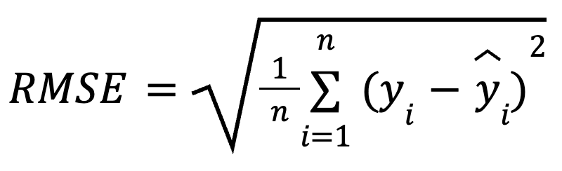
here:

• y_i is the actual value for observation i,
• _ŷ, is the predicted value for observation i,
• n is the total number of observations.

By squaring the residuals before averaging, RMSE penalizes larger errors more heavily than smaller ones. This sensitivity makes it a good choice when large prediction mistakes are especially undesirable. RMSE is always non-negative, and lower values indicate a better-fitting model.

Three Equal Ways to Calculate RMSE

RMSE is easy to compute. It’s simply a matter of calculating the residuals, squaring them, finding the mean, and taking the square root.

Let’s consider a few different ways to calculate it.

Using residuals

In this method, we start by subtracting predictions from the actual values to get the residuals. Next, we square each residual, average all of them, and finally take the square root.

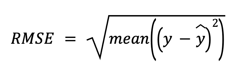
here:

• y is the vector of actual values,
• ŷ, is the vector of predicted values.

This direct approach emphasizes the prediction errors themselves.

Using mean squared error (MSE)

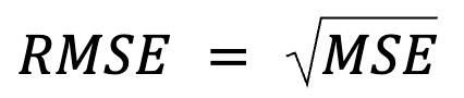
This one feels just like a restatement, but really there’s more to it: RMSE is simply the square root of the MSE. 

where:

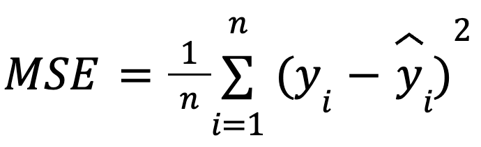
with:

• y_i as the actual value for observation i,
• ŷ, as the predicted value for observation i,
• n as the total number of observations.

This formulation is useful because MSE is a common loss function in model optimization. This equivalence is especially important in machine learning, where MSE is often the loss function minimized during training via gradient descent. 

More on this: It is precisely because RMSE introduces a square root that many machine learning algorithms choose not to RMSE during model training. MSE is preferred for these optimizations because it has simpler derivatives (again, because the square root introduces nonlinearity). RMSE is then often used post hoc to report performance in interpretable units.

In matrix form

In multiple regression, RMSE can also be derived from the residual vector using matrix algebra:

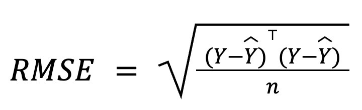
where:

• Y is the column vector of actual values,
• ŷ is the column vector of predicted values,
• n is the number of observations.

This matrix-based formulation is particularly compact and computationally efficient, especially for large datasets or model pipelines. We have a dedicated linear algebra course if you want to study the math.

Interpreting RMSE

RMSE is interpreted as the average prediction error, which determines the model’s prediction accuracy. Put simply, it shows, on average, how far the predictions are from the actual values, in the same scale as the outcome variable.

A lower RMSE suggests smaller average prediction errors and, hence, more accurate predictions, but the “acceptable” RMSE depends entirely on the context. For example, an RMSE of 2 might be good when predicting almond size in millimeters, but not so compelling when predicting annual almond crop yields in tons.

To be meaningful, RMSE should be compared across models trained on the same data or through benchmarking on historical performance.

When to Use RMSE

RMSE is particularly helpful in these scenarios:

• When absolute prediction accuracy is key
• When comparing models on the same dataset
• When model errors are normally distributed
• When our goal is to minimize large errors
• When interpreting errors in natural units is important

However, RMSE has its downsides:

• It’s sensitive to outliers. A few large residuals can disproportionately affect the RMSE and make it misleading.
• It isn’t normalized. This means that it can’t compare across different datasets and target scales unless the target variable is scaled.

RMSE Examples in Python and R

Let’s now illustrate how to calculate RMSE in both Python and R using the Ice-Cream Sales Dataset from Kaggle. We’ll build two models in each programming language and then compute RMSE for each model:

• Model 1: Uses the relevant predictor (temperature).
• Model 2: Adds a random, irrelevant predictor.

Python example

Let’s start with Python.

import pandas as pd
import numpy as np
from sklearn.linear_model import LinearRegression
from sklearn.metrics import mean_squared_error

# Load dataset
df = pd.read_csv("Ice Cream.csv")

# Extract features and target
X = df[['Temperature']]
y = df['Revenue']

# Model 1
model1 = LinearRegression()
model1.fit(X, y)
pred1 = model1.predict(X)
rmse1 = np.sqrt(mean_squared_error(y, pred1))
print(f"Model 1 RMSE: {rmse1:.3f}")

# Model 2 with an irrelevant predictor
np.random.seed(0)
df['Noise'] = np.random.normal(0, 1, size=len(df))
X2 = df[['Temperature', 'Noise']]

model2 = LinearRegression()
model2.fit(X2, y)
pred2 = model2.predict(X2)
rmse2 = np.sqrt(mean_squared_error(y, pred2))
print(f"Model 2 RMSE: {rmse2:.3f}")

Model 1 RMSE: 24.915
Model 2 RMSE: 24.911

We can see that RMSE for Model 2 is very similar to Model 1. While Model 2 may seem more complex, its actual prediction accuracy can worsen since we just included random noise that adds no useful information.

To level up your regression skills in Python, enroll in these courses:

• Introduction to Regression with statsmodels in Python
• Intermediate Regression with statsmodels in Python

R example

Now, let’s try in R.

# Load dataset
df <- read.csv("Ice Cream.csv")

# Model 1
model1 <- lm(Revenue ~ Temperature, data = df)
pred1 <- predict(model1, df)
rmse1 <- sqrt(mean((df$Revenue - pred1)^2))
cat("Model 1 RMSE:", round(rmse1, 3), "\n")

# Model 2 with an irrelevant predictor
set.seed(0)
df$Noise <- rnorm(nrow(df), mean = 0, sd = 1)
model2 <- lm(Revenue ~ Temperature + Noise, data = df)
pred2 <- predict(model2, df)
rmse2 <- sqrt(mean((df$Revenue - pred2)^2))
cat("Model 2 RMSE:", round(rmse2, 3), "\n")

Model 1 RMSE: 24.915 
Model 2 RMSE: 24.915

Here I've refashioned the same example in R. RMSE stayed exactly the same when we included an irrelevant predictor. This confirms that RMSE may not always change when adding noise variables, especially if the model assigns them negligible weight. However, complexity still increases, and the model could generalize worse on new data.

You might have noticed a small difference between the two examples: In Python, RMSE decreased slightly after adding the irrelevant predictor, while in R, RMSE stayed the same. This happened because the random noise generated in each environment (even though I made sure it was drawn from the same distribution) was not identical.

If you had trouble getting your R code to compile, or if you had trouble interpreting the result, try our courses:

• Introduction to Regression in R
• Intermediate Regression in R

RMSE vs. Related Metrics

RMSE is part of a broader family of regression error metrics. Let’s briefly compare it to others, clarify the differences between them, and highlight when each is most useful.

RMSE vs. MAE

RMSE penalizes large errors more heavily because it squares the residuals, making it more sensitive to outliers. MAE (mean absolute error), by contrast, is more robust to outliers, treats all errors equally, and works better for measuring typical error size when outliers are not a concern. While RMSE minimizes squared loss, MAE minimizes absolute loss.

In general, we should use RMSE when large errors can be especially costly, and MAE when we want a median-like view of error, less sensitive to outliers.

RMSE vs. R-squared

RMSE provides the average error in original units, which makes it more intuitive for practical interpretation. Instead, R-squared describes how much variance is explained by the model but doesn’t indicate prediction error size.

They are often used together: R-squared for relative fit, and RMSE for absolute performance.

RMSE vs. MSE

RMSE is just the square root of MSE, making it easier to interpret because it’s in the same units as the outcome variable. 

Aside from just interpretation, however, MSE is especially useful for optimization during training for machine learning. Remember that if you optimized on RMSE, the square root function means the model would put more emphasis on larger errors. Also, MSE has a smooth derivative, so it works well with gradient-based algorithms like stochastic gradient descent, enabling efficient convergence during model training. In short, RMSE is easier to interpret because we are looking at results on the scale of the data, but we should know that deep learning often optimizes MSE, not RMSE.

RMSE vs. MAPE

MAPE (mean absolute percentage error) returns errors as percentages, which is handy for comparing across datasets. However, it breaks down when actual values are close to zero, making it unstable. RMSE avoids this issue and is more reliable when small target values are present.

RMSE vs. log-likelihood

Here’s another interesting relationship: RMSE is formally equivalent to the negative log‑likelihood under Gaussian errors. Or rather, we should maybe say that minimizing RMSE is equivalent to maximizing the log-likelihood (of a regression model) under the assumption of normally distributed errors (with constant variance). I'm not saying that RMSE by itself estimates the full log-likelihood, but I am saying that minimizing RMSE implicitly maximizes the log-likelihood under a normal error assumption.

However, when errors are skewed or have outliers, alternatives like Huber or quantile loss may perform better. In any case, we should treat our metric choice as a model‑design decision, not an afterthought.

Common Misconceptions About RMSE

Let’s clarify some widespread myths about RMSE:

• “A low RMSE guarantees good generalization of the model.” This is not necessarily true. A model can have a low value of RMSE on the training data but still perform poorly on new, unseen data due to overfitting. To assess generalization efficiently, we need to conduct cross-validation or use a separate test set.
• “RMSE can determine if a model is overfitting.” RMSE alone can’t do it. It must be compared between training and validation datasets: if the training RMSE is low but the validation RMSE is much higher, that means overfitting.
• “There’s a fixed universal threshold for a good RMSE.” No, there isn’t. Whether the value of RMSE is “good” depends entirely on the context, domain, and units of the outcome variable. In other words, RMSE values are meaningless without context.

Conclusion

To wrap up, RMSE is a practical, interpretable, and intuitive measure of prediction accuracy that communicates average prediction error in the units of the target variable. It’s a go-to metric for regression performance evaluation, especially when error magnitudes matter.

However, RMSE should be used alongside other metrics such as R-squared, MAE, and cross-validation scores to get a fuller picture of model quality. We shouldn’t rely on this measure blindly but always consider scale, context, and model complexity. In addition, pairing RMSE with visual diagnostics can help detect bias. 

In short, RMSE tells us how wrong our model is, on average, in real terms, which is a powerful perspective to keep when building predictive systems.

If anything in this article was confusing, don’t worry. We have many great resources to help: 

• Simple Linear Regression: Everything You Need to Know tutorial
• Understanding Sum of Squares: A Guide to SST, SSR, and SSE tutorial
• Introduction to Regression with statsmodels in Python course
• Introduction to Regression in R course