

Q-Q Plots and Other Diagnostic Plots
If you are familiar with linear model diagnostic plots, you may also know that there are quite a few options to assess model fit. In order to understand exactly what the Q-Q plot is showing, let’s look at a few other diagnostics. This will help us better understand what the Q-Q plot is doing and what other plots might complement it.
- Fitted Values versus Residuals: This plot shows the relationship between the predicted values (fitted values) and the residuals, which are the differences between the observed and predicted values.
- Histogram of Residuals: This plot shows the distribution of the residuals.
- Scale-Location Plot: This plot shows the relationship between the residuals and the fitted values.
- Leverage versus Standardized Residuals: This plot highlights how far a data point is in the predictor space and whether the model fits it well or poorly. We standardize the residuals to evaluate their relationship with leverage on a consistent scale.
- Observation Number versus Cook’s Distance: This plot identifies specific data points with the highest overall influence on the model by combining leverage and residual size. The observation number on the x-axis serves as an identifier for each data point.
- Leverage versus Cook’s Distance: This plot compares a point's potential to influence the model with its actual overall impact on model predictions.
I'll show you quickly how to create each plot using tidyverse methods. The purpose here is not to interpret the linear model from our “Cars in Jordan” dataset for every linear model diagnostic on this list. Rather, I want to show the other diagnostic plots so you can recognize them, use the code if it is helpful, and, to the point of this article, so you can better situate the Q-Q plot among the other diagnostic plots. This way, you will understand better what the Q-Q plot is showing and not showing, how it is helpful, and what it is missing.
fitted_values_vs_residuals <- ggplot(data = car_linear_model, aes(x = .fitted, y = .resid)) +
geom_point(color = '#203147') +
geom_hline(yintercept = 0, linetype = "dashed", color = '#01ef63', size = 1) +
xlab("fitted values") +
ylab("residuals") +
labs(title = "Cars in Jordan") +
labs(subtitle = "Fitted Values vs Residuals")
histogram_of_residuals <- ggplot(data = car_linear_model, aes(x = .resid)) +
geom_histogram(color = '#01ef63') +
xlab("residuals") +
labs(title = "Cars in Jordan") +
labs(subtitle = "Histogram of Residuals")
scale_location <- ggplot(car_linear_model, aes(.fitted, sqrt(abs(.stdresid)))) +
geom_point(color = '#203147', na.rm=TRUE) +
stat_smooth(method="loess", na.rm = TRUE, color = '#01ef63', size = 1, se = FALSE) +
xlab("Fitted Value") +
ylab(expression(sqrt("|Standardized residuals|"))) +
labs(title = "Cars in Jordan") +
labs(subtitle = "Scale-Location")
leverage_vs_standardized_residuals <- ggplot(data = car_linear_model, aes(.hat, .stdresid)) +
geom_point(aes(size = .cooksd), color = '#203147') +
stat_smooth(method="loess", na.rm=TRUE, color = '#01ef63', size = 1) +
xlab("Leverage") +
ylab("Standardized Residuals") +
labs(title = "Cars in Jordan") +
labs(subtitle = "Residuals vs Leverage") +
scale_size_continuous("Cook's Distance", range=c(1,5)) +
theme(legend.title = element_blank()) +
theme(legend.position= "none")
observation_number_vs_cooks_distance <- ggplot(car_linear_model, aes(seq_along(.cooksd), .cooksd)) +
geom_bar(stat="identity", position="identity", color = '#01ef63', size = 1) +
xlab("Obs. Number") +
ylab("Cook's distance") +
labs(title = "Cars in Jordan") +
labs(subtitle = "Cook's distance")
leverage_vs_cooks_distance <- ggplot(car_linear_model, aes(.hat, .cooksd))+geom_point(na.rm=TRUE) +
stat_smooth(method="loess", na.rm=TRUE, color = '#01ef63', size = 1) +
xlab("Leverage hii")+
ylab("Cook's Distance") +
labs(title = "Cars in Jordan") +
labs(subtitle = "Cook's dist vs Leverage hii/(1-hii)") +
geom_abline(slope=seq(0,3,0.5), color = "gray", linetype = "dotdash")
library(patchwork)
fitted_values_vs_residuals + histogram_of_residuals
library(patchwork)
scale_location + leverage_vs_standardized_residuals
library(patchwork)
observation_number_vs_cooks_distance + leverage_vs_cooks_distance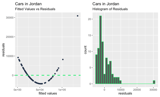
Fitted values versus residuals; histogram of residuals. Image by Author
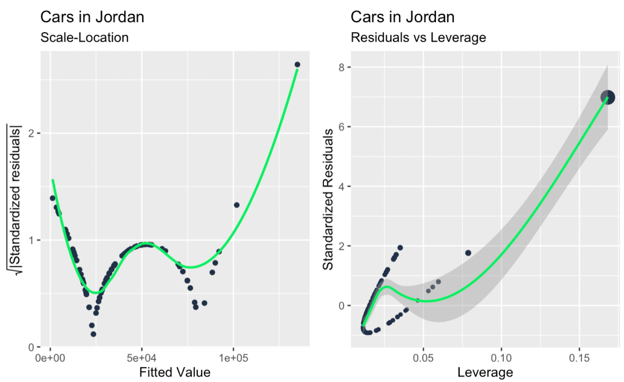
Scale-location plot; leverage versus standardized residuals. Image by Author
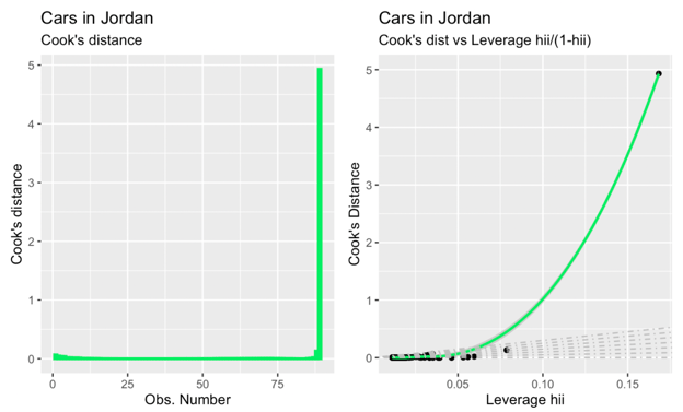
Observation number versus Cook's distance; Cook's distance versus leverage. Image by Author
Maybe the main takeaway, glancing at all the extra diagnostic plots above, is that there are one or two large outliers that are having a big impact on the slope of the regression line, and these outliers are not so obvious when glancing only at the Q-Q plot. So the Q-Q plot in our example serves its function - testing the normality of residuals - and also reveals a limitation, which is that it doesn't address independence, homoscedasticity, or outliers.
For additional reference, I'm including here a high-level table showing which linear model assumption is tested with each diagnostic plot, and I'm also suggesting how other diagnostic plots might work in tandem with the Q-Q plot. Keep in mind that, depending on the data, different kinds of patterns can be revealed with different diagnostic plots, and certain other things might be revealed in combination. For example, a Q-Q plot might confirm normality, while a scale-location plot could identify heteroscedasticity, and you might only see normality and heteroscedasticity by using both plots.
| Diagnostic Plot Type | Helps With | How it Works with the Q-Q Plot |
|---|---|---|
| Q-Q Plot | Normality of residuals | |
| Histogram of Residuals | Normality of residuals | Provides a quick visual and a general sense of symmetry and spread. |
| Fitted Values versus Residuals | Linearity, independence of errors | Reveals patterns and non-linearity, complementing the Q-Q plot’s normality check. |
| Scale-Location Plot | Homoscedasticity | Highlights residual spread consistency, complementing Q-Q plots for normality checks. |
| Leverage versus Residuals Plot | Independence of errors | Focuses on high-leverage points, which Q-Q plots do not address. |
| Observation Number versus Cook’s Distance | Identifying influential points | Complements Q-Q plots by locating outliers with high influence. |
| Leverage versus Cook’s Distance Plot | Identifying high-leverage points | Highlights influential observations, while Q-Q plots validate normality. |
Final Thoughts
I hope you have a new appreciation for Q-Q plots as a useful tool in assessing normality and have a better understanding of its common use in assessing the normality of residuals in a linear regression. I also hope that you have a new appreciation for the idea and importance of linear model diagnostics more generally.
Keep learning about linear regression with our Multiple Linear Regression in R: Tutorial With Examples which covers more complex models involving multiple predictors, including ideas of multicollinearity in regression. I strongly suggest enrolling in our full and comprehensive career track, Machine Learning Scientist in Python, to learn all about the model-building workflow, including both supervised and unsupervised learning.

Autor
Josef Waples
I'm a data science editor with contributions to research articles in scientific journals. I'm especially interested in linear algebra, statistics, R, and the like.
Q-Q Plot FAQs
What is a Q-Q plot?
A Q-Q plot, or Quantile-Quantile plot, is a visual tool used to compare the distribution of a dataset to a theoretical distribution, such as the normal distribution.
Is a Q-Q plot the same as a normal Q-Q plot?
A normal Q-Q plot is a type of Q-Q plot where one dataset is compared to a normal distribution with specified parameters. It is used to assess whether a dataset follows a normal distribution. So, all normal Q-Q plots are Q-Q plots, but not all Q-Q plots are normal Q-Q plots.



Linear regression models are widely used in statistics and machine learning to predict numerical values based on input features, and also to understand the relationship between variables. However, just because you can fit a line through your data doesn't mean you should. We have to also diagnose the quality of the fit to determine if the model is appropriate for the data or if it needs to be refined.
There are a few different ways to test a model, including evaluating the model using a train/test workflow and looking at model statistics like adjusted r-squared. In this article, I will focus on how to create and interpret a specific diagnostic plot called the Q-Q plot, and I will show you a few different methods to create this Q-Q plot in the R programming language. To really continue mastering regression techniques, take Introduction to Regression in R or Intermediate Regression in R or, for Python, take Introduction to Regression in Python or Intermediate Regression in Python, depending on your level of comfort.
What is a Q-Q Plot?
A Q-Q (Quantile-Quantile) plot is used to see if a dataset follows a particular theoretical distribution. It works by comparing the quantiles of the observed data to the quantiles of this other distribution. I said ‘theoretical distribution’ to be exact, but often when we create a Q-Q plot, we really think of the normal, or Gaussian, distribution specifically, and we refer to it as a normal Q-Q plot. However, Q-Q plots can also be used to compare data against other distributions, such as exponential, uniform, chi-squared, t-distribution, Poisson distribution, or others, depending on the context.
It's helpful to understand by showing an example. Here, I've created 10 numbers. To construct a normal Q-Q plot, I first put the numbers in order. I then calculate the probability with this equation: q = (i– 0.5)/n. Then, I could use the percent-point function (PPF) of the standard normal distribution (the
qnorm()function) to find the corresponding value for the rank. (You might be more familiar with the cumulative distribution function (CDF), which tells us the probability up to a value x. Well, the PPF is like the opposite: It gives us the x-value for a given probability.)Finally, to create the graph, we plot the quantiles of our observed values against the theoretical quantiles (hence the two Qs in Q-Q plot). The line is constructed by calculating the slope and intercept using the first and third quartiles of both the observed and theoretical distributions.
Illustrative Q-Q plot. Image by Author
Why Use a Q-Q Plot?
A Q-Q plot is a nice visual way to check for distributional assumptions. There are other ways to test if data follows a normal distribution, like the Shapiro-Wilk test, for example, but nothing, in my opinion, is really quite so visual, and makes the story so obvious, as the Q-Q plot.
Knowing the distribution of something is important in a few ways. For one, we will probably want to know the best measures for center and spread. Also, when creating a linear regression, we want to know if our dependent variable, in particular, follows a normal distribution, and we also want to see if the residuals from our model are normally distributed so that we have better confidence in our estimates. So basically, I think Q-Q plots are useful for two general reasons: comparing our data to sample distributions and testing for normality.
How to Create a Q-Q Plot in R
Let’s look now at how to create a Q-Q plot in R. For this section, I will go through three different methods: base R, the
carpackage, and tidyverse methods. I think you will see that I prefer tidyverse methods because it gives you more flexibility to make the graph look nicer and it has more extensibility with other packages.For each method, I will create a Q-Q plot on the residuals of a simple linear regression, which is one of the most common uses - if not the most common use - of the Q-Q plot. However, you could also create a Q-Q plot to check the distribution of the variables before you create a linear regression in the first place. All you need is the distribution of one variable and a theoretical distribution to compare it with.
If you want to follow along, you can download the Kaggle dataset I’m using: Car Prices Jordan 2023.
Creating a Q-Q plot in base R
Let’s first create a Q-Q plot in base R, which is to say that we won’t be installing any extra packages but using only the built-in functions.
Creating a Q-Q plot using the car package
Now, let’s try creating a Q-Q plot using the
carpackage. In my opinion, the quality of the visualization is not too different, but this Q-Q plot does have the advantage that is shows a confidence envelope, which defines the area within which our data points are expected to lie if the model assumption of normality were to hold true.Creating a Q-Q plot using ggplot2
Now let’s look at how to create a Q-Q plot using tidyverse methods for more flexibility and to make it look nicer. This time around, I’m going to put the Q-Q plot as a panel next to my original scatterplot.
Linear regression and a Q-Q plot of the residuals created in ggplot2. Image by Author
What a Q-Q Plot Can Tell Us
With a Q-Q plot, the observed data's quantiles are plotted against the theoretical quantiles. If the data closely follows the theoretical distribution, the points on the Q-Q plot will move on a diagonal line. Deviations from this line indicate departures from the expected distribution. Points that fall above or below the line suggest skewness or outliers, and patterns such as curves or s-shaped deviations indicate systematic differences, like heavier or lighter tails.
There are about three things that we look for.
Let’s show with an example for each:
Three Q-Q plots: one with a straight line; one with a curve; one with a heavy tail. Image by Author
In the first case, the Q-Q line matches up with the data points, so the distribution is indeed normal. In the second case, we see a curved pattern, so the data is either not normal or else it is skewed. In the last case, we see a sort of ‘s’ shape, so the distribution has heavy tails or more extreme values.
Q-Q Plots in Linear Regression
There are a few different linear model assumptions, including linearity (that the relationship between variables is linear), independence of errors (that the errors are not correlated with each other), homoscedasticity (that the residuals should have constant variance), and normality of residuals (that the residuals follow a normal distribution). The Q-Q plot helps in particular with that fourth linear model assumption, the normality of residuals.
Here's how different patterns affect the interpretation and reliability of our model:
Straight Line Alignment
Curved Patterns
Heavy or Light Tails