Action Value Function: A Guide With Python Examples

Implementing an Action-Value Function

Having discussed the basic principles and uses of the action-value function, I now show you the steps to implement it in Python.

Step 1: Define the environment

Import the prerequisite packages, including Gymnasium and NumPy: 

import gymnasium as gym
import numpy as np
import math
import random

Initialize an RL environment from Gymnasium. In this article, we train an RL agent to solve the CartPole environment. 

env = gym.make('CartPole-v1')

Step 2: Initialize Q-table

The CartPole observation space has four states: cart position, cart velocity, pole angle, and pole angular velocity. 

In this example, we focus only on the pole angle and the pole angular velocity observations. Thus, we create the discrete Q-table as follows: 

• One discrete state for the cart position - all possible values get bucketed into this single state. 
• One discrete state for the cart velocity 
• Six discrete states for the pole angle
• Three discrete states for the pole velocity 

The number of columns is based on the size of the action space, in this case, 2. 

NUM_BUCKETS = (1, 1, 6, 3)
NUM_ACTIONS = env.action_space.n
q_table = np.zeros(NUM_BUCKETS + (NUM_ACTIONS,))

In the CartPole environment, the state-space is continuous. The cart pole's angle, velocity, and position can vary continuously. The action-space is discrete - you can push the cart to the left or the right. 

Q-Learning using Q-tables can only be used on a discrete space because you need to explicitly tabulate the Q-value for a set of states and actions. So, the first step is to discretize the continuous state space. 

We first consider the upper and lower bounds of the state space variables. We notice that the cart velocity and pole angular velocity have infinite bounds. So, we artificially set upper and lower bounds on these state variables. 

STATE_BOUNDS = list(zip(env.observation_space.low, env.observation_space.high))
STATE_BOUNDS[1] = [-0.5, 0.5]
STATE_BOUNDS[3] = [-math.radians(50), math.radians(50)]

We create a function to discretize the continuous state values into discrete ones: 

def discretize_state(state):
    discrete_states = []

    for i in range(len(state)):
        if state[i] <= STATE_BOUNDS[i][0]:
            discrete_state = 0
        elif state[i] >= STATE_BOUNDS[i][1]:
            discrete_state = NUM_BUCKETS[i] - 1
        else:
            bound_width = STATE_BOUNDS[i][1] - STATE_BOUNDS[i][0]
            offset = (NUM_BUCKETS[i] - 1) * STATE_BOUNDS[i][0] / bound_width
            scaling = (NUM_BUCKETS[i] - 1) / bound_width
            discrete_state = int(round(scaling * state[i] - offset))
        discrete_states.append(discrete_state)
    return tuple(discrete_states)

Step 3: Update the Q-table

The Bellman equations give the expression to update the Q-values based on the learning rate, the discount rate, the reward going into the next step, and the expected maximal Q-value of the next state. It expresses the expected value of a state as the sum of two parts: 

• The immediate reward going into the next state
• The discounted expected value of the next state 

The Bellman equation is recursive. Thus, it is possible to write an iterative program, starting from a random initial state, to find the optimal action-value function. 

The equation for updating the Q-table is: 

In the expression above: 

• The current state is s_t, denoted as state_current in the code.
• The next state is s_t+1 (state_next).
• The action taken in the current state is at (action).
• Q(s_t, a_t) is the current Q-value for the state s_t and action a_t
• α is the learning rate.
• γ is the discount factor.
• r_t+1 is the reward after taking action a_t in the current step with state s_t. The code below represents this as reward. 
• argmax_a Q(s_t+1, a) is the maximum Q-value of the next state s_t+1. In the code snippet below, this is represented at best_q. 

The code below implements the function to update the Q-table

def update_q(state_current, state_next, action, reward, alpha):
    best_q = np.amax(q_table[state_next])
    q_table[state_current + (action,)] += alpha * (reward + GAMMA*(best_q) - q_table[state_current + (action,)])
    return best_q

Step 4: Train the agent

Declare the parameters of the training: 

• The maximum number of training episodes
• The maximum number of steps per episode comes from the environment’s documentation. For CartPole-v1, it is 500. 
• The number of steps the agent should complete for the episode to be classified as a success. We set it at 450. 
• The number of successful episodes the agent should complete in a row to consider the training successful. We set it at 50. 

MAX_EPISODES = 5000
MAX_STEPS = 500
SUCCESS_STEPS = 450
SUCCESS_STREAK = 50

Declare the hyperparameters:

• The minimum and maximum values of the exploration rate, ε
• The minimum and maximum values of the learning rate, α
• The rate of decay of α and γ
• The discount factor, γ

EPSILON_MIN = 0.01
EPSILON_MAX = 1
ALPHA_MIN = 0.1
ALPHA_MAX = 0.5
GAMMA = 0.99
DECAY_COEFF = 25

Before training the agent, we write two functions to decay the learning rate and the exploration rate gradually. These hyperparameters decrease in value gradually throughout the training. 

def decay_epsilon(step):
    return max(EPSILON_MIN, min(EPSILON_MAX, 1.0-math.log10((step+1)/DECAY_COEFF)))

def decay_alpha(step):
    return max(ALPHA_MIN, min(ALPHA_MAX, 1.0-math.log10((step+1)/DECAY_COEFF)))

We also write a function to select the action stochastically. We first generate a random number. 

• If this random number is less than ε, we randomly choose an action from the action space. This is the exploration strategy. 
• If the random number is greater than ε, we choose the action corresponding to the maximum Q-value. This is the exploitative strategy. 

def select_action(state, epsilon):
    if random.random() < epsilon:
        action = env.action_space.sample()
    else:
        action = np.argmax(q_table[state])
    return action

We build a loop to train the agent based on the following steps:

• Fetch the decayed values of α and ε for the current episode.
• Reset the environment and discretize the observation space to start a fresh environment for the episode. 
• Run the agent in the environment till it reaches the maximum number of steps or terminates. 
• For each step:
• Select the action according to the select_action() function declared earlier. 
• Run the action on the environment to get the reward and the next state. 
• Get the highest Q-value from the Q-table. 
• Update the Q-table according to the update_q() function declared earlier. 

The code below implements the steps of the training loop:

def train():
    successful_episodes = 0
    for episode in range(MAX_EPISODES):
        epsilon = decay_epsilon(episode)
        alpha = decay_alpha(episode)
        observation, _ = env.reset()
        state_current = discretize_state(observation)
        for step in range(MAX_STEPS):
            action = select_action(state_current, epsilon)
            observation, reward, terminated, truncated, _ = env.step(action)
            done = terminated or truncated
            state_next = discretize_state(observation)
            best_q = update_q(state_current, state_next, action, reward, alpha)
            state_current = state_next
            if done:
                print("Episode %d finished after %d time steps" % (episode, step))
                print("best q value: %f" % (float(best_q)))
                if (step >= SUCCESS_STEPS):
                    successful_episodes += 1
                    print("=============SUCCESS=============")
                else:
                    successful_episodes = 0
                    print("=============FAIL=============")
                break
            if successful_episodes > SUCCESS_STREAK:
                break

Finally, run the training loop, close the environment, and print the final value of the Q-table. 

train()
env.close()
print(q_table)

Use this DataLab workbook as a starting point to edit and execute the code for Q-Learning. 

Extending to Deep Q-Learning

In the previous section, we discretized the continuous (state) observation space to use a Q-table. A large Q-table (for complex environments) is computationally inefficient. In such cases, the Q-function can be approximated using a neural network. This is called a Deep Q-Network, expressed as Q(s, a; θ), where the parameter θ represents the weights of the neural network. This method is called Deep Q-learning. More generally, RL using deep neural networks is called Deep Reinforcement Learning. 

Instead of using the Q-Table to choose the action for each state, the DQN neural network takes the state as input and returns the Q-value for each possible action in that state. 

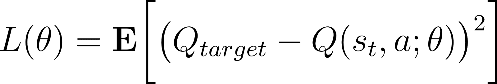
The network is trained via traditional methods (like backpropagation) to minimize the temporal difference (TD) error. The TD error δ is the difference between the predicted Q-values and the target Q-values (calculated as the sum of the reward from the current state and the discounted value of the expected maximum reward from the next state). 

When implemented as a neural network (with network parameters θ), the TD error is expressed as:

Notice that both Q-values and the target Q-values are calculated using the same neural network. 

In each iteration, the network parameters (θ) are updated. The network update (via backprop) is based on the target value computed using the pre-update θ. Calculating the target values with the same updated results in a continuously moving target. This makes the training unstable. 

To avoid the above problem, we create a new network to calculate the target Q values. This is the target network. It is based on the same parameters as the policy network but it is updated less frequently. Thus, the training process has a stable target with respect to which it applies backpropagation. 

If we represent the weights of the target network with θ^-, the earlier equation is restated as:

The following sections will show how to implement and train a simple DQN in the CartPole environment. 

Example implementation

Install the prerequisite packages, including Gymnasium and PyTorch. 

!pip install gymnasium matplotlib torch

Import the necessary packages in the Python environment: 

import gymnasium as gym
import math
import random
import matplotlib
import matplotlib.pyplot as plt
from collections import namedtuple, deque
from itertools import count

import torch
import torch.nn as nn
import torch.optim as optim
import torch.nn.functional as F

Create the CartPole environment: 

env = gym.make("CartPole-v1")

Initialize the environment and declare Python constants with the size of the environment’s state and action spaces. 

state, info = env.reset()
NUM_OBSERVATIONS = len(state)
NUM_ACTIONS = env.action_space.n

Declare a Python class for a simple neural network with a single hidden layer. The number of input layers is the size of the state space (observation space). The number of output layers is the number of possible actions the RL agent can take. This network internally simulates the Q-table and predicts the action values given an input state. 

class DQN(nn.Module):

    def __init__(self, NUM_OBSERVATIONS, NUM_ACTIONS):
        super(DQN, self).__init__()
        self.layer1 = nn.Linear(NUM_OBSERVATIONS, 128)
        self.layer2 = nn.Linear(128, 128)
        self.layer3 = nn.Linear(128, NUM_ACTIONS)

    def forward(self, x):
        x = F.relu(self.layer1(x))
        x = F.relu(self.layer2(x))
        return self.layer3(x)

Create a policy network and a target network. Load the target network with the policy network’s parameters using the state dictionary. Initialize an optimizer to train the neural network. 

policy_net = DQN(NUM_OBSERVATIONS, NUM_ACTIONS)
target_net = DQN(NUM_OBSERVATIONS, NUM_ACTIONS)
target_net.load_state_dict(policy_net.state_dict())

optimizer = optim.AdamW(policy_net.parameters(), lr=LR, amsgrad=True)

Training with replay buffer

Off-policy model-free RL methods such as Q-Learning (discussed in the previous section) and DQNs are trained using a random sample of the agent’s interactions with the environment. The agent’s actions and the environment’s responses (reward and next state) are collected and stored. A random sample of these interactions is picked in each training iteration to form a training batch. 

Declare a tuple object to store the environment’s state (observation) in each interaction:

Transition = namedtuple('Transition', ('state', 'action', 'next_state', 'reward'))

Create a Python class for the replay buffer:

class ReplayMemory(object):

    def __init__(self, capacity):
        self.memory = deque([], maxlen=capacity)

    def push(self, *args):
        self.memory.append(Transition(*args))

    def sample(self, batch_size):
        return random.sample(self.memory, batch_size)

    def __len__(self):
        return len(self.memory)

Create a memory object to store a large number of interactions. These interactions are used to train the agent. 

memory = ReplayMemory(10000)

Before training, declare the parameters and hyperparameters:

• Parameters: 
• Batch size
• Maximum number of training episodes
• Hyperparameters:
• Learning rate (LR)
• Discount factor (GAMMA)
• The update rate of the target network (TAU)
• Initial and final values of the exploration rate, and the rate of decay (EPS_START, EPS_END, and EPS_DECAY)

MAX_EPISODES = 600
BATCH_SIZE = 128

GAMMA = 0.99
EPS_START = 0.9
EPS_END = 0.05
EPS_DECAY = 1000
TAU = 0.005
LR = 1e-4

Write a function to select the action based on the exploration rate, based on these steps:

• Calculate the exploration rate based on the number of steps in the episode (and the initial and final values and decay rate of the exploration rate). 
• Generate a random number. 
• If the random number is greater than the exploration rate, choose the action predicted by the policy network. 
• If it is less than the exploration rate, choose a random action from the action space. 

steps_done = 0
def select_action(state):
    global steps_done
    sample = random.random()
    eps_threshold = EPS_END + (EPS_START - EPS_END) * \
        math.exp(-1. * steps_done / EPS_DECAY)
    steps_done += 1
    if sample > eps_threshold:
        with torch.no_grad():
            action = policy_net(state).max(1).indices.view(1, 1)
            return action
    else:
        action = torch.tensor([[env.action_space.sample()]], dtype=torch.long)
        return action

Write the function to optimize the model based on these steps:

• Create a batch using a random sample of the agent’s interactions with the environment. Each item in the sample corresponds to one time step. It contains:
• The environment’s current state
• The agent’s action
• The reward received
• The next state
• In CartPole, the agent is expected to continue manipulating the cart pole without terminating (hitting the edges or falling). Thus, we consider only those interactions that do not lead to a terminal state. We create a mask (non_final_mask) to identify those states that are not followed by a terminal state. 
• Identify those states that are not followed by a terminal state (non_final_next_states).
• Get the state action values for all the current states s_t by passing the current states to the policy network. 
• Get the expected state action values for all the next states s_t+1 by passing the next states to the target network and using the equation:

• Calculate the loss based on the difference between the action values and the expected action values:

• Backpropagate the losses to calculate the gradients.
• Clip the gradient values and update the policy network to ensure stable training. 

The code below shows how to implement the optimizer:

batch = 0
def optimize_model():
    global batch
    if len(memory) < BATCH_SIZE:
        return
    transitions = memory.sample(BATCH_SIZE)
    batch = Transition(*zip(*transitions))

    non_final_mask = torch.tensor(tuple(map(lambda s: s is not None,
                                          batch.next_state)), dtype=torch.bool)
    non_final_next_states = torch.cat([s for s in batch.next_state
                                                if s is not None])
    state_batch = torch.cat(batch.state)
    action_batch = torch.cat(batch.action)
    reward_batch = torch.cat(batch.reward)

    state_action_values = policy_net(state_batch).gather(1, action_batch)
    next_state_values = torch.zeros(BATCH_SIZE )

    with torch.no_grad():
        next_state_values[non_final_mask] = target_net(non_final_next_states).max(1).values

    expected_state_action_values = (next_state_values * GAMMA) + reward_batch

    loss_func = nn.SmoothL1Loss()
    loss = loss_func(state_action_values, expected_state_action_values.unsqueeze(1))

    optimizer.zero_grad()
    loss.backward()

    torch.nn.utils.clip_grad_value_(policy_net.parameters(), 100)
    optimizer.step()

Write a training loop to train the agent:

• Reset the environment and start a new episode.
• Use the select_action() function to decide the agent’s action.
• Get the environment’s reward and next state based on the action.
• Append the state, action, next state, and reward to the replay buffer.
• Run the optimizer (defined above). The optimizer calculates the Q-values and the loss, applying backpropagation to update the network. 
• Update the target network based on the policy network.
• Continue the episode until it reaches a terminal state.

The following code implements these steps: 

def train():
    for episode in range(MAX_EPISODES):
        # Initialize the environment and get its state
        state, info = env.reset()
        state = torch.tensor(state, dtype=torch.float32).unsqueeze(0)
        for t in count():
            action = select_action(state)
            observation, reward, terminated, truncated, _ = env.step(action.item())
            reward = torch.tensor([reward])
            done = terminated or truncated

            if terminated:
                next_state = None
            else:
                next_state = torch.tensor(observation, dtype=torch.float32).unsqueeze(0)

            memory.push(state, action, next_state, reward)
            state = next_state
            optimize_model()

            target_net_state_dict = target_net.state_dict()
            policy_net_state_dict = policy_net.state_dict()
            for key in policy_net_state_dict:
                target_net_state_dict[key] = policy_net_state_dict[key]*TAU + target_net_state_dict[key]*(1-TAU)
            target_net.load_state_dict(target_net_state_dict)

            if done:
                episode_durations.append(t + 1)
                print('episode -- ', episode)
                print('count -- ', t)
                #plot_durations()
                break

You can view, edit, and run the DQN training program using this DataLab workbook. 

Visualizing the Action-Value Function

It is useful to visually track the progress of the training process. Visualizing the action values helps to recognize where the training is failing and what parameters or hyperparameters need to be changed. 

For example, if you visually observe that the improvement in the model’s performance is too slow, you might want to increase the learning rate. If you notice that the model is learning but hasn’t been fully trained yet, it might help to increase the number of training episodes. If you find the training to be unstable, you might want to reduce the learning rate or tweak the exploration coefficient, or the update rate of the target network (TAU). 

In addition to the Q-values, it can also help to plot the number of successful steps in each episode. In Q-Learning using Q-tables, the Q-values are explicitly stored. However, when using DQNs, the Q-values are not explicitly stored. The network outputs the action depending on its weights and the state. So, tracking the number of successful steps in each episode can be more meaningful for DQN. 

The following steps describe how to plot the Q-values and the number of successful steps per episode for training the Q-learning algorithm:

• Create two empty arrays at the start of the training:
• q_vals - for storing Q-values in each step of each episode. 
• success_steps - for storing the number of successful steps in each episode.
• At each step (in all the episodes):
• Append the Q-value for that step to the q_vals array
• After each episode terminates, append to the success_steps array the number of successful steps in that episode. 
• Plot both arrays. 

The code below shows the Q-Learning (using Q-tables) training loop (shown in the previous section) updated for tracking the Q-values and number of successful steps:

q_vals = []
success_steps = []

def train():
    global q_vals 
    global success_steps
    successful_episodes = 0

    for episode in range(MAX_EPISODES):
        epsilon = decay_epsilon(episode)
        alpha = decay_alpha(episode)
        observation, _ = env.reset()
        state_current = discretize_state(observation)

        for step in range(MAX_STEPS):
            action = select_action(state_current, epsilon)
            observation, reward, terminated, truncated, _ = env.step(action)
            done = terminated or truncated
            state_next = discretize_state(observation)
            best_q = update_q(state_current, state_next, action, reward, alpha)
            q_vals.append(best_q)
            state_current = state_next

            if done:
                q_vals.append(best_q)
                success_steps.append(step)
                print("Episode %d finished after %d time steps" % (episode, step))
                print("best q value: %f" % (float(best_q)))
                if (step >= SUCCESS_STEPS):
                    successful_episodes += 1
                else:
                    successful_episodes = 0
                break

            if successful_episodes > SUCCESS_STREAK:
                print("Training successful")
                return

The snippet below shows how to plot the Q-values in each episode:

def plot_q():
    plt.plot(q_vals)
    plt.title('Q-values over training steps')
    plt.xlabel('Training steps')
    plt.ylabel('Q-value')
    plt.show()

The following snippet shows how to plot the number of successful steps in each episode:

def plot_steps():
    plt.plot(success_steps)
    plt.title('Successful steps over training episodes')
    plt.xlabel('Training episode')
    plt.ylabel('Successful steps')
    plt.show()

• The DataLab workbook for implementing Q-learning using action-value functions also includes the code to plot the Q-values and successful steps per episode. 
• The notebook for implementing DQN also includes the code to plot the number of successful steps per episode. 

Evaluating agent performance

It is necessary to specify the criteria for deciding whether and when the agent has been successfully trained. In traditional ML, the goal of training is to minimize the loss: the difference between the predicted and true values. In RL, the goal is to maximize the cumulative reward. The training is considered successful when the agent obtains the maximum rewards from the environment. 

Environments like CartPole do not end until they reach a terminal condition, like hitting the edges or allowing the cartpole to lean excessively. In such cases, a trained agent can continue interacting with the environment indefinitely. Thus, the maximum number of successful steps is artificially imposed. In the case of Gymnasium’s CartPole-v1, the episode is terminated when it reaches 500 timesteps without terminating. 

We evaluate the agent’s performance over consecutive episodes to evaluate whether the training is successful. For example: 

• The agent should be able to complete more than a threshold number of steps (SUCCESS_STEPS) on average over the last N episodes. In the examples in this article, we set this threshold at 450. 
• The agent can cross the threshold in N consecutive episodes (SUCCESS_STREAK). In this example, we set N at 50. 

As a practical example, consider this snippet from the DQN training loop shown previously. 

if done:
  episode_durations.append(t + 1)
  print('episode -- ', episode)
  average_steps = sum(episode_durations[-SUCCESS_STREAK:])/SUCCESS_STREAK
  print('average steps over last 50 episodes -- ', average_steps)
  if average_steps > SUCCESS_STEPS:
      print("training successful.")
      return
  break

It helps to evaluate the agent’s performance based on executing the following steps at the end (terminal state) of every training episode:

• Append the total number of steps in this episode (before it ended) to an array. This array tracks the total number of steps in each episode. 
• Calculate the average of the last N values in this array. In this example, N (SUCCESS_STREAK) is 50. So, we calculate the average steps over the last 50 episodes. 
• If this average is greater than a threshold (SUCCESS_STEPS), we end the training. In this example, this threshold is set at 450 steps. 

Best Practices for Using Action-Value Functions

Here are some best practices you can follow for better results from your action-value function implementation. 

Balance exploration and exploitation

Given the true action-value function, the agent can maximize expected returns by adopting a greedy strategy, based on choosing the action with the highest value at each step. This is called exploitation of the available information. However, using a greedy strategy with an untrained action-value function (which does not yet represent the true action-values) will lead to getting stuck in a local optima. 

During training, it is important to both explore the environment and exploit the available information. 

In the initial stages of the training process, the available information is based on a random value function. Hence, this information is not very valuable (to exploit with a greedy strategy). It is more important to explore the environment to discover the rewards from various possible actions in different states. 

As the Q-table is updated (or the DQN is trained), it becomes viable to partially exploit the available information to maximize the rewards. Towards the final stages of the training, the agent converges on the true value function; further exploration can be detrimental. Hence, the agent prioritizes exploiting the known value function. 

Tune hyperparameters

As with any machine learning model, hyperparameters are important for successfully training RL algorithms. In the case of Q-Learning and DQNs, the hyperparameters are epsilon (exploration rate), alpha (learning rate), and gamma (discount rate). 

• ε (epsilon) controls the balance of exploration and exploitation (discussed above). The higher the epsilon value, the more important exploration is relative to exploitation. At the start of the training, it takes on a high value like 0.9, which is gradually reduced to a small value like 0.05 towards the end of the training.
• α (alpha) is the learning rate (LR). It controls how much the parameters of the neural network (in the case of DQNs) or the values of the Q-Table change in each training iteration. If the LR is too high, the model becomes unstable and fails to converge. On the other hand, a low LR leads to slow convergence. It is also common to start with a high value of the LR early in the training process when the agent needs to explore the environment. As it gets closer to the true values of the Q-function, the LR is reduced to help the network converge.
• γ (gamma) is the discount rate. It decides the importance of rewards in later timesteps over immediate rewards. A high value of gamma means that later rewards are important.  A gamma value of 0 means that only the reward from the current time step is important, and later rewards hold no significance. In algorithms like Q-learning, the total return is based on rewards earned throughout the entire episode. So, using a high discount rate, like 0.99, is common.

Lastly, understand that RL training is sensitive to initial random values. If the training doesn’t converge, it is often helpful to use a different random seed or re-run the training so it starts with a different set of random initial values. 

Start with simple environments

Training RL agents for complex environments is challenging. Q-functions are used in many different algorithms, so it is essential to build some intuition for training Q-learning-based RL agents. This is best done by practicing the techniques on simpler environments like CartPole before applying similar methods to more complex environments. 

Furthermore, complex environments are more costly to train in, so it is more economical to use simpler environments as a learning tool. 

Conclusion

This article discussed the fundamental theoretical principles of the action value function and its significance in RL. We covered how action value functions are used in Q-learning and Deep Q-learning, and implemented both these methods step-by-step in Python.

To continue your learning, I highly recommend the Deep Reinforcement Learning in Python course.