Course
One of the most important things that you'll want to do when you're performing a network analysis is determining the centrality of a node within a social network. In other words, if you have a network for analysis, you'll want to figure out which node has the most effect on the others. This tutorial will cover exactly that. In it, you'll learn more about the following topics:
- What is the definition of centrality?
- What are the types of centrality measures?
- What is the process of designating the best centrality measure according to the network topology?
The Definition of Centrality
Nowadays, learning how to find basic nodes of a network is vital for every researcher who wants to work on network science. As you go forward, networks in the context of different sciences come to be more enormous and complex. Therefore, meticulously analyzing each node is costly and time-consuming and somehow impossible. Centrality description answers the question: "Which node is the most important one in the network?".
A function that assigns a numerical value to each vertex of a network according to its influence on the others. The importance of a node is determined by its position within a network. Depending on the type of the network, you can describe what importance means. It could be identified as an effective person in a social network or key infrastructure nodes in the urban networks.
Centrality Measures: Types
Centrality indices can be classified in local and global categorizes.
Local Centrality Measures
An example of a local centrality measure is the degree centrality, which counts the number of links held by each node and points at individuals who can quickly connect with the wider network. It is a local measure since it does not take into account the rest of the network and the importance you give to its value depends strongly on the network's size.
To calculate popular centrality measures like degree, you can use igraph package. You can make it available with the help of the library() function:
library(igraph)Before you perform any centrality calculation, you need to have a network. To do this, you can use one of the random algorithms, such as the Erdos-Renyi model, to build the sample graph.
The Erdos-Renyi model was introduced by Paul Erdos and Alfred Renyi, two greatest mathematician, in 1959. It is useful to generate random graphs in which each pair of nodes are connected by equal probability value to form an edge. In this model of random graphs, most of the nodes have approximately equal number of connections and the degree distribution of the model is usually binomial or Poisson. This can be used in the probabilistic methods to prove the existence of graphs with diverse properties, or to elaborate a comparison in terms of structure with real networks.
To see an example of the Erdos-Renyi model, you can use sample_gnm() function from the igraph package.
# n = number of nodes, m = the number of edges
erdos.gr <- sample_gnm(n=10, m=25)

plot(erdos.gr)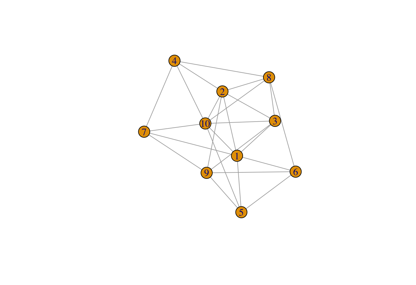
It is an undirected network, a graph with bidirectional edges in contrast with a directed graph in which the direction of an edge from one vertex to another is considered, with 10 nodes and 25 edges.
The degree centrality of this graph would be calculated using centr_degree() function:
degree.cent <- centr_degree(erdos.gr, mode = "all")
degree.cent$res

##  [1] 2 3 5 6 7 7 6 3 6 5
As illustrated, node 1 has the highest degree centrality values through all in the sample network.
Global Centrality Measures
Global centrality measures, on the other hand, take into account the whole of the network. One of the most widely used global centrality measures is closeness centrality. This measure scores each node based on their closeness to all other nodes within the network.
It calculates the shortest paths between all nodes, then assigns each node a score based on its sum of shortest paths and is useful for finding the individuals who are best placed to influence the entire network most quickly.
It is recommended to use Closeness to find central vertices within a single cluster. You can calculate this via the closeness() function in the igraph package.
closeness.cent <- closeness(erdos.gr, mode="all")
closeness.cent

##  [1] 0.05882353 0.06250000 0.07142857 0.08333333 0.09090909 0.09090909
##  [7] 0.08333333 0.06250000 0.08333333 0.07692308
According to the closeness centrality results, unlike degree centrality, nodes 1 and 9 have the highest centrality values through the whole network. This means that these nodes have equally important roles in the flow of the network.
How to Pick the Best Centrality Measure
Although there are different types of centrality measures to determine the most influential nodes of a network, there's not yet a consensus pipeline in network science to select and implement the best tailored measure for a given network.
For the illustration, the following plot demonstrates the scatter plot between two centrality measures named "subgraph centrality" and "topological coefficient". The red line indicates a strong negative association among the two centrality measures.
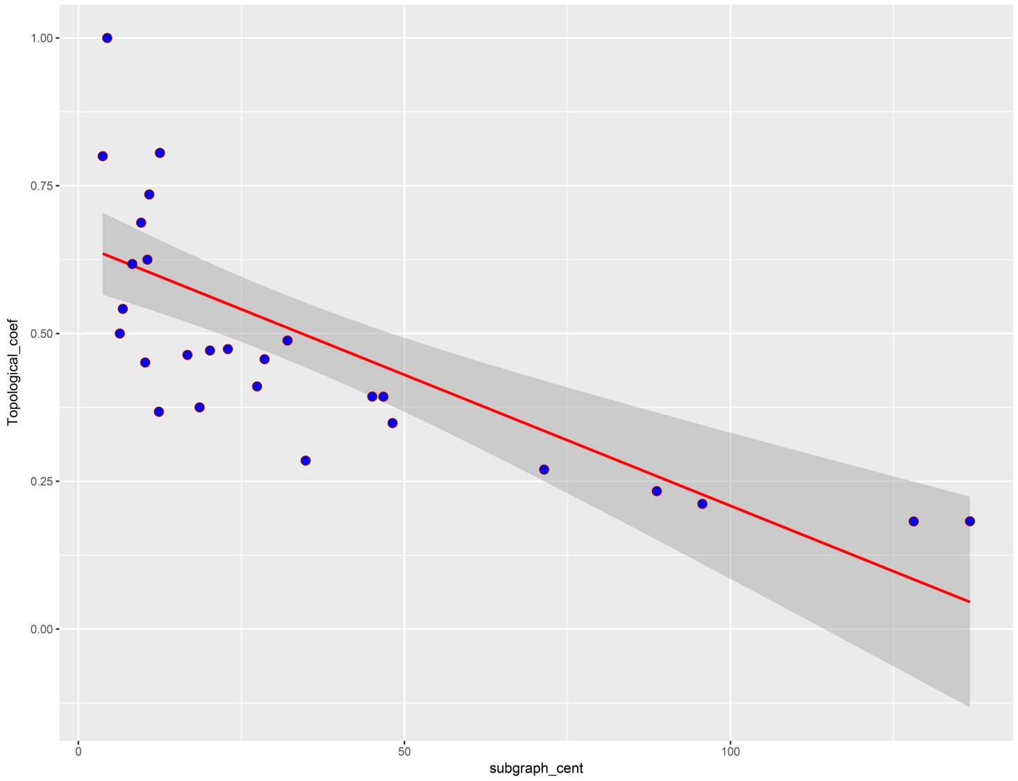
You can conclude from the above representation that as these two centralities have inverse relationships, they can distinguish the central nodes within a network based on different patterns and so the result of centrality calculation would be variant according to the centrality type.
There are more than 140 benchmarks currently available to identify the central vertices, but which one should be used to calculate the influential nodes?
Additionally, as the topological features of a network effects on the result of the centrality calculations, you have to select a criterion that has the highest level of information about the influential vertices based on the network topoly.
CINNA (Central Informative Nodes in Network Analysis) is an R package for computing, analyzing and comparing centrality measures submitted to CRAN repository.
To see how you can use this package, you start by using one of the data sets inside the package called Zachary. This data set illustrates friendships among members of a university karate club:
library(CINNA)

data("zachary")

plot(zachary)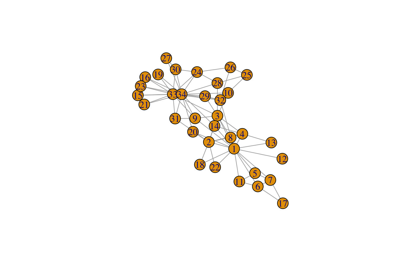
This is an undirected graph, with 34 vertices and 78 edges. Remember that an undirected graph is one where your edges have no orientation: they are bi-directional. For example: A<--->B == B<--->A.
To figure out the calculable centrality types based on the graph structure, the proper_centralities() function can be useful.
pr_cent<-proper_centralities(zachary)

##  [1] "subgraph centrality scores"
##  [2] "Topological Coefficient"
##  [3] "Average Distance"
##  [4] "Barycenter Centrality"
##  [5] "BottleNeck Centrality"
##  [6] "Centroid value"
##  [7] "Closeness Centrality (Freeman)"
##  [8] "ClusterRank"
##  [9] "Decay Centrality"
## [10] "Degree Centrality"
## [11] "Diffusion Degree"
## [12] "DMNC - Density of Maximum Neighborhood Component"
## [13] "Eccentricity Centrality"
## [14] "eigenvector centralities"
## [15] "K-core Decomposition"
## [16] "Geodesic K-Path Centrality"
## [17] "Katz Centrality (Katz Status Index)"
## [18] "Kleinberg's authority centrality scores"
## [19] "Kleinberg's hub centrality scores"
## [20] "clustering coefficient"
## [21] "Lin Centrality"
## [22] "Lobby Index (Centrality)"
## [23] "Markov Centrality"
## [24] "Radiality Centrality"
## [25] "Shortest-Paths Betweenness Centrality"
## [26] "Current-Flow Closeness Centrality"
## [27] "Closeness centrality (Latora)"
## [28] "Communicability Betweenness Centrality"
## [29] "Community Centrality"
## [30] "Cross-Clique Connectivity"
## [31] "Entropy Centrality"
## [32] "EPC - Edge Percolated Component"
## [33] "Laplacian Centrality"
## [34] "Leverage Centrality"
## [35] "MNC - Maximum Neighborhood Component"
## [36] "Hubbell Index"
## [37] "Semi Local Centrality"
## [38] "Closeness Vitality"
## [39] "Residual Closeness Centrality"
## [40] "Stress Centrality"
## [41] "Load Centrality"
## [42] "Flow Betweenness Centrality"
## [43] "Information Centrality"
The outcome contains a list indicating 43 popular centrality names specific for an undirected-unweighted structure.
Let's choose the first five centrality measures out of the list and pass them to the calculate_centralities() function, because computations of the all calculable centralities would be time-consuming.
In the next step, you use the Principal Component Analysis (PCA) algorithm to distinguish the most informative centrality measure.
Remember that PCA is a dimensional reduction technique respectively for linear analysis.
In this step of analysis, each centrality measure plays as a variable. Hence, centralities which are correlated with the principal components are the most important in identifying the central nodes. The contribution criterion from the PCA shows how variables contribute to the principal components.
In the other words, the contributions of variables accounts the variability relative to principal components(in percentage). Thanks to this criterion in the PCA method, you can detect which centralities have more information about the central nodes and so, which one can describe influential vertices of a network more accurately. Therefore, sorted contribution indices of centralities can be visualized like below.
In the following, you will apply these two recent steps consecutively using a pipe operator %>%:
calculate_centralities(zachary, include = pr_cent[1:5])%>%
  pca_centralities(scale.unit = TRUE)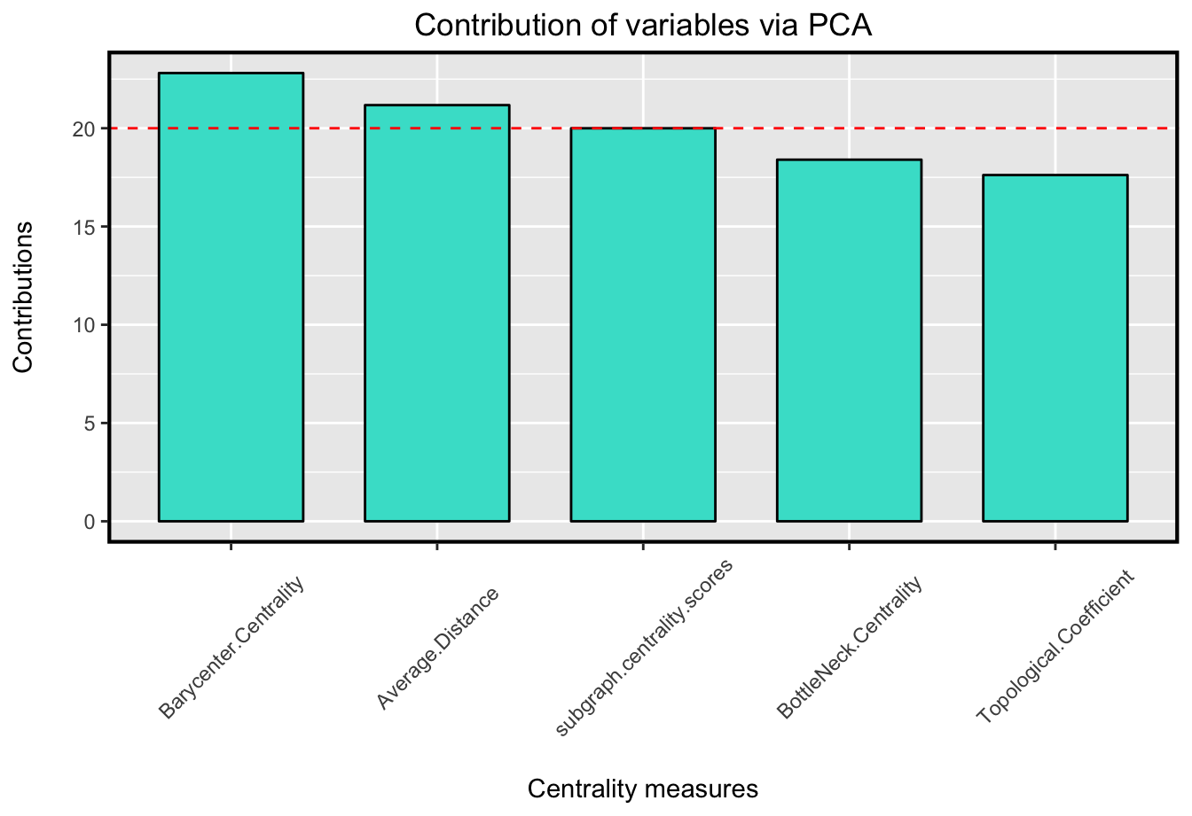
As it's shown in the plot, Barycenter Centrality has the most contribution value among the five centrality indices.
In other words, it has the most information about the influential nodes among the computed centrality measures. Hence, it can determine the central nodes more accurately than the chosen centrality.
A representation of the graph in which each nodes size indicates its corresponding centrality value, would be like below.
visualize_graph( zachary , centrality.type="Barycenter Centrality")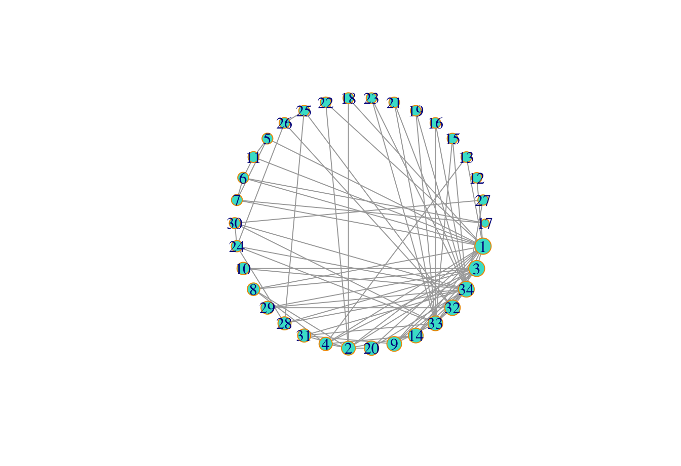
Accordingly, node 1 is the most central node through all.
Wrap-up
All in all, in order to quantify the connectivity of a network, it is recommended to apply PCA on some centrality measures which you can calculate according to the network structure and pick the most informative one to compute and to explain the maximum contribution amount relative to their corresponding principal components.
In this tutorial, you first depicted the centrality definition and talked about some popular ones. Then, you emphasized that, as the global properties of a network would affect the central component detection, the influential nodes of a network would be different, depending on the network topology.
In the next step, you used the CINNA package, which provided all necessary functions for applying centrality analysis within a network. With this package, you were able to operate the centrality analysis on your network without any additional work. Furthermore, this increased the accuracy of central nodes determination significantly.
If you'd like to dive right in the subject and see how it works, check out this paper, and also this one.
For any questions or concerns about the matter above, please do not hesitate to contact me on Minoo_Ashtiani.
To learn more about R, check out our Basic Programming Skills in R tutorial and the following courses:

