Course
K-means is a popular unsupervised machine learning technique that allows the identification of clusters (similar groups of data points) within the data. In this tutorial, you will learn about k-means clustering in R using tidymodels, ggplot2 and ggmap. We'll cover:
- how the k-means clustering algorithm works
- how to visualize data to determine if it is a good candidate for clustering
- a case study of training and tuning a k-means clustering model using an Airbnb review dataset
Before going deeper, we recommend you brush up on your basics of R Programming, such as vectors and data frames. If you are instead ready for this journey, skip it and let’s start!
Develop AI Applications
An Overview of k-Means Clustering
Clustering models aim to group data into distinct “clusters” or groups. This can be used an analysis by itself, or can be used as a feature in a supervised learning algorithm.
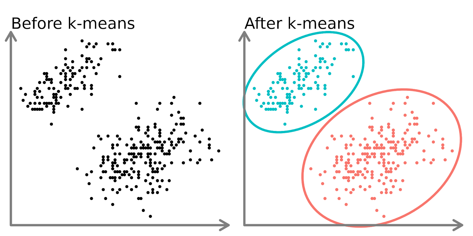
In the left-hand side of the diagram above, we can see 2 distinct sets of points that are unlabeled and colored as similar data points. Fitting a k-means model to this data (right-hand side) can reveal 2 distinct groups (shown in both distinct circles and colors).
In two dimensions, it is easy for humans to split these clusters, but with more dimensions, you need to use a model.
The k-means algorithm
Imagine you want to create several fruit salads, each consisting of similar fruits.
- You decide on the number of fruit salads you want to create (k). For instance, you decide to make 3 fruit salads.
- You randomly choose 3 fruits from the table as the starting "representatives" of each salad.
- Now, you go around the table and assign each fruit to the salad whose representative it most resembles. For instance, apples might go with pears, oranges with tangerines, and bananas with plantains.
- Once all the fruits have been assigned, you find the new "center" of each fruit salad by calculating the average fruit characteristics in each group (e.g., size, color, taste). These new centers become the updated representatives.
- You repeat steps 3 and 4 several times, assigning fruits to the most similar representative and updating the representative each time until the groupings no longer change.
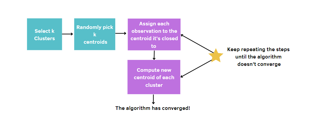
More generally, you:
- Choose the number of clusters, k.
- Select k points (clusters of size 1) at random.
- Calculate the distance between each point and the centroid and assign each data point to the closest cluster.
- Calculate the centroid (mean position) for each cluster.
- Keep repeating steps 3–4 until the clusters don’t change or the maximum number of iterations is reached.
Since k-means picks randomly the centers of the clusters, this algorithm needs to be run a certain number of times, which is fixed by the user. In this way, the best solution will be reached, by minimizing a model quality’s measurement. This measurement is called the total within-cluster sum of squares (WCSS), that is the sum of the distances between the data points and the corresponding centroid for each cluster. Indeed, the more our model quality measurement is small, the more we’ll reach the winning model.
Airbnb Listings Dataset
All the content of this tutorial will revolve around Airbnb rental listings in Cape Town, available on DataLab. The data contains different types of information, like the hosts, the price, the number of reviews, the coordinates and so on.
Even if the dataset seems to provide deep information about vacation rentals, there are still some clear questions that can be answered. For example, let’s imagine that Airbnb requests to its data scientists to investigate the segmentation of the listings within this platform in Cape Town.
Every town is different from the other and has different exigences depending on the culture of the people living there. The identification of clusters in this city may be useful to extract new insights, that can increase the satisfaction of actual customers with suitable Customer Loyalty Strategies, avoiding customer churn. At the same time, it’s also crucial to attract new people with appropriate promotions.
Visualize Airbnb data
Before applying k-means, we would like to investigate more on the relationship between the variables by taking a look at the correlation matrix. For convenience of display, we round the digits to two decimal places.
library(dplyr)
airbnb |>
  select(price, minimum_nights, number_of_reviews) |>
  cor(use = "pairwise.complete.obs") |>
  round(2)
From the output, there seems to be a slight negative relationship between price and the number of reviews: The higher the price, the lower the number of reviews. The same for minimum nights and a number of reviews. Since the minimum nights don’t have a big impact on the price, we would just like to investigate more on how price and number of reviews are related:
library(ggplot2)
ggplot(data, aes(number_of_reviews, price, color = room_type, shape = room_type)) +
    geom_point(alpha = 0.25) +
    xlab("Number of reviews") +
    ylab("Price")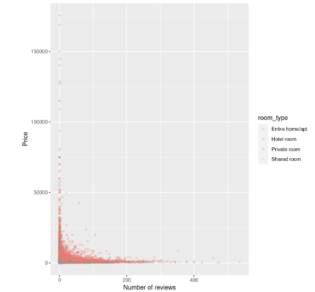
The scatterplot shows that the cost of accommodations, in particular entire houses, is higher when there is a small number of reviews, and seems to decrease as the number of reviews grows.
Normalization
Before fitting the model, there is a further step to do. k-means is sensitive to variables that have incomparable units, leading to misleading results. In this example, the number of reviews is tens or hundreds, but the price is tens of thousands. Without any data processing, the differences in price would appear to be larger than differences in reviews, but we want these variables to be treated equally.
To avoid this problem, the variables need to be transformed to be on a similar scale. In this way, they can be compared correctly using the distance metric.
There are different methods to tackle this issue. The most known and used is standardization, which consists in subtracting the average value from the feature value and, then, dividing it by its standard deviation. This technique will allow obtaining features with a mean of 0 and a deviation of 1.
You can scale the variables with the scale() function. Since this returns a matrix, the code is cleaner using a base-R style rather than a tidyverse style.
airbnb[, c("price", "number_of_reviews")] = scale(airbnb[, c("price", "number_of_reviews")])Fitting and evaluating the model
We can finally identify the clusters of listings with k-means. For getting started, let’s try performing k-means by setting 3 clusters and nstart equal to 20. This last parameter is needed to run k-means with 20 different random starting assignments and, then, R will automatically choose the best results total within-cluster sum of squares. We also set a seed to replicate the same results every time we run the code.
# Get the two columns of interest
airbnb_2cols <- data[, c("price", "number_of_reviews")]

set.seed(123)
km.out <- kmeans(airbnb_2cols, centers = 3, nstart = 20)
km.out
Output:
K-means clustering with 3 clusters of sizes 785, 37, 16069

Cluster means:
     price number_of_reviews
1 14264.102         5.9401274
2 83051.541         0.6756757
3  1589.879        18.2649200

Clustering vector:
   [1] 3 3 3 3 3 3 3 3 1 3 3 3 3 3 3 3 3 1 3 3 3 3 3 3 3 3 3 3 3 3 3 3 3 3 3 3
  [37] 3 3 3 3 3 3 3 3 3 3 3 3 3 3 3 3 3 3 3 3 3 3 3 3 3 3 3 3 3 3 3 3 3 3 3 3
  [73] 3 3 3 3 3 3 3 3 3 3 3 3 3 3 3 3 3 3 3 3 3 3 3 3 3 3 3 3 3 3 3 3 3 3 3 3
 [109] 3 3 3 3 3 3 3 3 3 3 3 3 3 3 3 3 3 3 3 3 3 3 1 3 3 3 3 3 3 3 3 3 3 3 3 3
 [145] 3 3 3 3 3 3 3 3 3 3 3 3 3 3 3 3 3 3 3 3 3 3 3 3 3 3 3 3 3 3 3 3 1 1 3 3
...
[16777] 3 3 3 3 3 3 3 3 3 3 1 3 3 1 3 1 3 3 3 3 3 1 3 3 3 3 3 3 3 3 1 3 3 3 3 3
[16813] 3 1 3 3 3 3 3 3 3 3 3 3 3 3 3 3 3 3 3 3 3 3 3 3 3 3 3 3 3 3 3 3 3 3 1 3
[16849] 3 3 3 3 3 3 3 3 3 3 3 3 3 3 3 3 3 3 3 3 3 3 3 3 1 3 3 3 3 3 3 3 3 3 3 3
[16885] 3 3 3 3 3 3 3

Within cluster sum of squares by cluster:
[1] 41529148852 49002793251 33286433394
(between_SS / total_SS =  74.5 %)

Available components:

[1] "cluster"      "centers"      "totss"        "withinss"     "tot.withinss"
[6] "betweenss"    "size"         "iter"         "ifault"
From the output, we can observe that three different clusters have been found with sizes 785, 37 and 16069. For each cluster, the squared distances between the observations to the centroids are calculated. So, each observation will be assigned to one of the three clusters.
Even if it seems like a good result, the best way to find the best model is to try different models with a different number of clusters. So, we need to start from a model with a single cluster, after we try a model with two clusters and so on. All this procedure needs to be tracked using a graphical representation, called scree plot, in which the number of clusters is plotted on the x-axis, while WCSS is on the y-axis.
In this case study, we build 10 k-means models, each of these will have a different number of clusters, reaching a maximum of 10 clusters. Moreover, we are going to use only a part of the dataset. So, we include only the price and the number of reviews. To plot the scree plot, we need to save the total within-cluster sum of squares of all the models into the variable wss.
# Decide how many clusters to look at
n_clusters <- 10

# Initialize total within sum of squares error: wss
wss <- numeric(n_clusters)

set.seed(123)

# Look over 1 to n possible clusters
for (i in 1:n) {
  # Fit the model: km.out
  km.out <- kmeans(airbnb_2cols, centers = i, nstart = 20)
  # Save the within cluster sum of squares
  wss[i] <- km.out$tot.withinss
}

# Produce a scree plot
wss_df <- tibble(clusters = 1:n, wss = wss)

scree_plot <- ggplot(wss_df, aes(x = clusters, y = wss, group = 1)) +
    geom_point(size = 4)+
    geom_line() +
    scale_x_continuous(breaks = c(2, 4, 6, 8, 10)) +
    xlab('Number of clusters')
scree_plot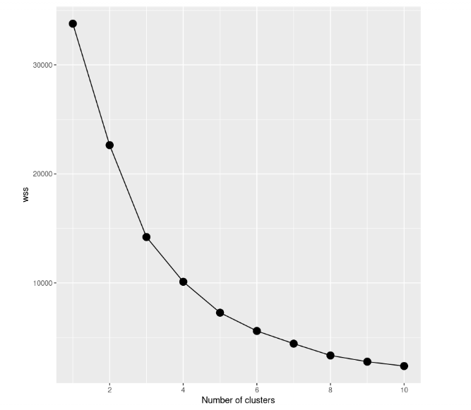
By taking a look at the scree plot, we can notice how the total within-cluster sum of squares decreases as the number of clusters grows. The criterion to choose the number of clusters is by finding an elbow such that you are able to find a point where the WCSS decreases much slower after adding another cluster. In this case, it’s not so clear, so we’ll add horizontal lines to get a better idea:
scree_plot +
    geom_hline(
        yintercept = wss,
        linetype = 'dashed',
        col = c(rep('#000000',4),'#FF0000', rep('#000000', 5))
    )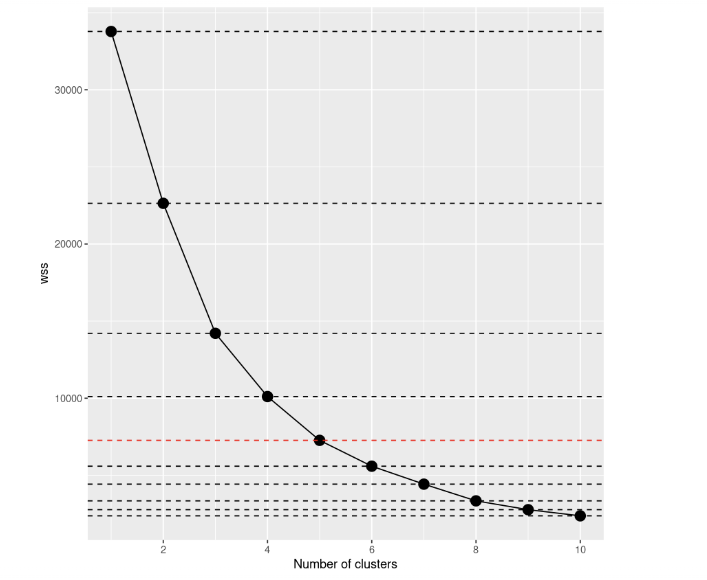
If you take a look again, the decision to make seems much more clear than before, don’t you think? From this visualization, we can say that the best choice is to set up the number of clusters equal to 5. After k=5, the improvements of the models seem to reduce sharply.
# Select number of clusters
k <- 5
set.seed(123)
# Build model with k clusters: km.out
km.out <- kmeans(airbnb_2cols, centers = k, nstart = 20)
We can try again to visualize the scatterplot between the price and the number of reviews. We also colour the points based on the cluster id:
data$cluster_id <- factor(km.out$cluster)
ggplot(data, aes(number_of_reviews, price, color = cluster_id)) +
    geom_point(alpha = 0.25) +
    xlab("Number of reviews") +
    ylab("Price")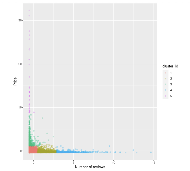
We can observe that:
- There are a few listings that have high prices and low reviews, coloured in green and fuchsia
- We also have a group of data points with both low prices and reviews, marked in red
- After that, the price seems to stabilize as soon as the number of reviews increases.
When will K-Means fail?
Keep attention that k-means is simple and easy to apply, but it’s not always the best choice to segment data into groups since it may fail. There is the assumption that the clusters are spherical and, then, it does a good job with these cases, while groups with different sizes and densities tend not to be captured well by this algorithm.
When these conditions are not respected, it’s preferable to find other alternative approaches, like DBSCAN and BIRCH. Clustering in Machine Learning: 5 Essential Clustering Algorithms provides a great overview of clustering approaches in case you want to dig deep.
Take it to the Next Level
We can conclude that k-means remains one of the most used clustering algorithms to identify distinct subgroups, even if it’s not always perfect in all situations. Now, you have the knowledge to apply it with R in other case studies
If you want to want to study deeper this method more, take a look at the course Unsupervised Learning in R. There is also Cluster Analysis in R and An Introduction to Hierarchical Clustering in Python to have a complete overview of the clustering approaches available, which can be useful when k-means isn’t enough to provide meaningful insights from your data. In case you also want to explore supervised models with R, this course is recommended!

