PyTorch CNN Tutorial: Build and Train Convolutional Neural Networks in Python

Convolutional Neural Networks (CNNs) are a cornerstone of modern computer vision, enabling applications such as image recognition, facial detection, and self-driving cars. These networks are designed to automatically extract patterns and features from images, making them more powerful than traditional machine learning techniques for visual tasks.

In this tutorial, we will implement a CNN using PyTorch, a deep learning framework that is both user-friendly and highly efficient for research and production applications.

Prerequisites: Deep Learning and PyTorch

Before getting into the details of CNNs, you must be familiar with the field of deep learning and the Python libraries we will use during the setup of our environment.

Deep learning is a subset of machine learning, where the fundamental model structure is a network of inputs, hidden layers, and outputs. Such a network can have one or many hidden layers. The original intuition behind deep learning was to create models inspired by how the human brain learns: through interconnected cells called neurons. This is why we continue to call deep learning models "neural" networks. These layered model structures require far more data to learn than other supervised learning models to derive patterns from the unstructured data. We normally talk about at least hundreds of thousands of data points.

While there are several frameworks and packages out there for implementing deep learning algorithms, we'll focus on PyTorch, one of the most popular and well-maintained frameworks. In addition to being used by deep learning engineers in industry, PyTorch is a favored tool amongst researchers. Many deep learning papers are published using PyTorch. It is designed to be intuitive and user-friendly, sharing a lot of common ground with the Python library NumPy. 

If you need a primer on these concepts, consider enrolling in the Deep Learning with PyTorch course today. 

What is a Convolutional Neural Network (CNN)?

Convolutional neural networks, commonly called CNN or ConvNet, are a specific kind of deep neural network well-suited for computer vision tasks. The invention of CNNs dates back to the 1980s. However, they only became mainstream in the 2010s, following the computing breakthroughs that resulted from the implementation of graphics processing units (GPUs). Indeed, the rapid popularization of CNNs helped the field of neural networks regain prominence, leading to the so-called "third wave of neural networks" that we’re still living today.

CNNs are specifically inspired by the biological visual cortex. The cortex has small regions of cells that are sensitive to the specific areas of the visual field. This idea was expanded by a captivating experiment by Hubel and Wiesel in 1962. 

CNNs try to replicate this feature by creating complex neural networks that are made of different, task-specific layers. CNNs are called "feed-forward" because information flows right through the model. There are no feedback connections in which the outputs of the model are fed back into itself, compared to other models that use techniques like backpropagation.

In particular, a CNN typically consists of the following layers:

Convolutional layer

This is the first building block of a CNN. As the name suggests, the main mathematical task performed is called convolution, which is the application of a sliding window function to a matrix of pixels representing an image. The sliding function applied to the matrix is called kernel or filter. In the convolution layer, several filters of equal size are applied, and each filter is used to recognize a specific pattern from the image, such as the curving of the digits, the edges, the whole shape of the digits, and more. 

Activation function

Normally, a ReLU activation function is applied after each convolution operation. This function helps the network learn non-linear relationships between the features in the image, making the network more robust for identifying different patterns. It also helps to mitigate the vanishing gradient problems. 

Pooling layer

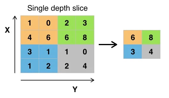
The goal of the pooling layer is to pull the most significant features from the convoluted matrix. This is done by applying some aggregation operations, which reduce the dimension of the feature map (convoluted matrix), thereby reducing the memory used while training the network.  Pooling is also relevant for mitigating overfitting.

Fully connected layers

These layers are in the last layer of the convolutional neural network, and their inputs correspond to the flattened one-dimensional matrix generated by the last pooling layer. ReLU activation functions are applied to them for non-linearity. 

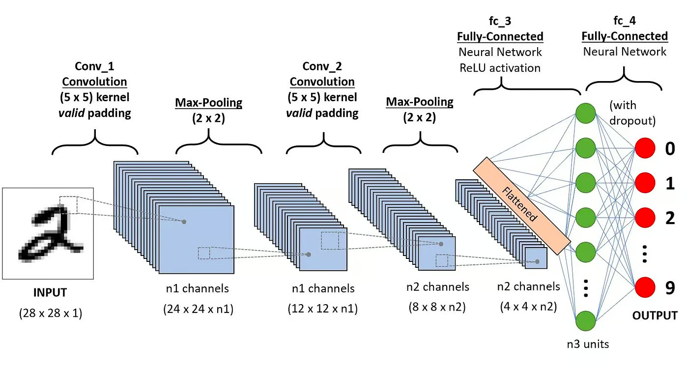Convolution Neural Network Architecture. Source: DataCamp

You can read a more detailed explanation of the maths behind CNNs in our tutorial, Convolutional Neural Networks in Python.

Why use CNNs for image classification?

Convolutional neural networks have been one of the most influential innovations in the field of computer vision. They have performed a lot better than traditional machine learning models, such as SVMs, and decision trees, and have produced state-of-the-art results. 

Furthermore, the convolutional layers grant CNNs their translation-invariant characteristics, empowering them to identify and extract patterns and features from data irrespective of variations in position, orientation, scale, or translation.


CNNs have proven to be successful in many different real-life case studies and applications, like:

• Image classification, object detection, segmentation, face recognition;
• Self-driving cars that leverage CNN-based vision systems;
• Classification of crystal structure using a convolutional neural network;
• Security camera systems.

Beyond image classification tasks, CNNs are versatile and can be applied to a range of other domains, such as natural language processing, time series analysis, and speech recognition.

Implementing a CNN with PyTorch

Now that you’re familiar with the theory of CNNs, we’re ready to get our hands dirty. In this section, we will build and train a simple CNN with PyTorch. Our goal is to build a model to classify digits in images. To train and test our model, we will use the famous MNIST dataset, a collection of 70,000 grayscale, 28x28 images with handwritten digits.

1. Importing required libraries

Below you can find the libraries we will use for this tutorial. In essence, we will leverage PyTorch to build our CNN, and PyTorch’s computer vision module torchvision, to download and load the MNIST dataset. Finally, we will also use torchmetrics to evaluate the performance of our model.

import numpy as np
import pandas as pd
import matplotlib.pyplot as plt


import torch
from torch import optim
from torch import nn
from torch.utils.data import DataLoader
from tqdm import tqdm

# !pip install torchvision
import torchvision

import torch.nn.functional as F
import torchvision.datasets as datasets
import torchvision.transforms as transforms

# !pip install torchmetrics
import torchmetrics

2. Loading and preprocessing the dataset

PyTorch also comes with a rich ecosystem of tools and extensions, including torchvision, a module for computer vision. Torchvision includes several image datasets that can be used for training and testing neural networks. In our tutorial, we will use the MNIST dataset. 

First, we will download and convert the MNIST dataset into a tensor, the core data structure in PyTorch, similar to NumPy arrays but with GPU acceleration capabilities.

Then, we'll also use DataLoader to handle batching and shuffling both the train and test datasets. A PyTorch DataLoader can be created from a Dataset to load data, split it into batches, and perform transformations on the data if desired. Then, it yields a data sample ready for training. In the code below, we load the data and save it in DataLoaders with a batch size of 60 images:

batch_size = 60

train_dataset = datasets.MNIST(root="dataset/", download=True, train=True, transform=transforms.ToTensor())

train_loader = DataLoader(dataset=train_dataset, batch_size=batch_size, shuffle=True)

test_dataset = datasets.MNIST(root="dataset/", download=True, train=False, transform=transforms.ToTensor())

test_loader = DataLoader(dataset=test_dataset, batch_size=batch_size, shuffle=True)

Optionally, the train dataset could be further split into two partitions of train and validation. Validation is a technique used in deep learning to evaluate model performance during training. It helps detect potential overfitting and underfitting of our models, and it’s particularly helpful to optimize hyperparameters. However, for the sake of simplicity, we won’t use validation for this tutorial. If you want to learn more about validation, you can check out a full explanation in our Introduction to Deep Learning with PyTorch Course.

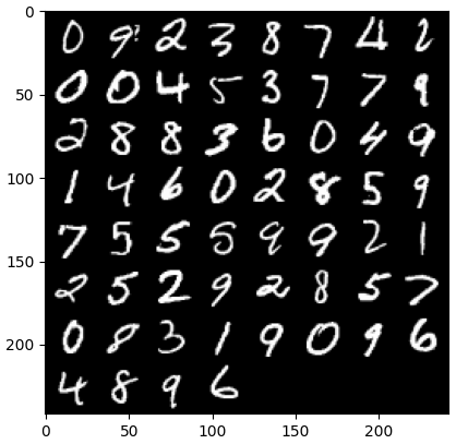
Now that we have our data, let’s see how a random batch of digits looks:

def imshow(img):
   npimg = img.numpy()
   plt.imshow(np.transpose(npimg, (1, 2, 0)))
   plt.show()

# get some random training images
dataiter = iter(dataloader_train)
images, labels = next(dataiter)
labels
# show images
imshow(torchvision.utils.make_grid(images))

3. Defining the CNN architecture

To solve the classification problem, we will leverage nn.Module class, PyTorch’s building block for intuitively creating sophisticated neural network architectures. 

In the code below, we create a class called CNN, which inherits the properties of nn.Module class. The CNN class will be the blueprint of a CNN with two convolutional layers, followed by a fully connected layer. 

In PyTorch, we use nn.Conv2d to define a convolutional layer. We pass it the number of input and output feature maps. We also set some of the parameters for the convolutional layer to work, including the kernel or filter size and padding. 

Next, we add a max pooling layer with nn.MaxPool2d. ​​In it, we slide a non-overlapping window over the output of the previous convolutional layer. At each position, we select the maximum value from the window to pass forward. This operation reduces the spatial dimensions of the feature maps, reducing the number of parameters and computational complexity in the network. Finally, we add a fully connected linear layer. 

The forward() function defines how the different layers are connected, adding several ReLU activation functions after each convolutional layer.

class CNN(nn.Module):
   def __init__(self, in_channels, num_classes):

       """
       Building blocks of convolutional neural network.

       Parameters:
           * in_channels: Number of channels in the input image (for grayscale images, 1)
           * num_classes: Number of classes to predict. In our problem, 10 (i.e digits from  0 to 9).
       """
       super(CNN, self).__init__()

       # 1st convolutional layer
       self.conv1 = nn.Conv2d(in_channels=in_channels, out_channels=8, kernel_size=3, padding=1)
       # Max pooling layer
       self.pool = nn.MaxPool2d(kernel_size=2, stride=2)
       # 2nd convolutional layer
       self.conv2 = nn.Conv2d(in_channels=8, out_channels=16, kernel_size=3, padding=1)
       # Fully connected layer
       self.fc1 = nn.Linear(16 * 7 * 7, num_classes)

   def forward(self, x):
       """
       Define the forward pass of the neural network.

       Parameters:
           x: Input tensor.

       Returns:
           torch.Tensor
               The output tensor after passing through the network.
       """
       x = F.relu(self.conv1(x))  # Apply first convolution and ReLU activation
       x = self.pool(x)           # Apply max pooling
       x = F.relu(self.conv2(x))  # Apply second convolution and ReLU activation
       x = self.pool(x)           # Apply max pooling
       x = x.reshape(x.shape[0], -1)  # Flatten the tensor
       x = self.fc1(x)            # Apply fully connected layer
       return x
       x = x.reshape(x.shape[0], -1)  # Flatten the tensor
       x = self.fc1(x)            # Apply fully connected layer
       return x

Once we have defined the CNN class, we can create our model and move it to the device where it will be trained and run. 

Neural networks, including CNNs, show better performance when running on GPUs, but that may be the case on your computer. Therefore, we will run the model on a GPU only when available; otherwise, we will use a regular CPU.

device = "cuda" if torch.cuda.is_available() else "cpu"

model = CNN(in_channels=1, num_classes=10).to(device)
print(model)
>>> CNN(
  (conv1): Conv2d(1, 8, kernel_size=(3, 3), stride=(1, 1), padding=(1, 1))
  (pool): MaxPool2d(kernel_size=2, stride=2, padding=0, dilation=1, ceil_mode=False)
  (conv2): Conv2d(8, 16, kernel_size=(3, 3), stride=(1, 1), padding=(1, 1))
  (fc1): Linear(in_features=784, out_features=10, bias=True)
)

4. Training the CNN model

Now that we have our model, it’s time to train it. To do so, we first will need to determine how we will measure the performance of the model. Since we are dealing with a multi-class classification problem, we will use the cross-entropy loss function, available in PyTorch as nn.CrossEntropyLoss. We will also use Adam optimizer, one of the most popular optimization algorithms. 

# Define the loss function
criterion = nn.CrossEntropyLoss()

# Define the optimizer
optimizer = optim.Adam(model.parameters(), lr=0.001)

We will iterate over ten epochs and training batches to train the model and perform the usual sequence of steps for each batch, as shown below.

num_epochs=10
for epoch in range(num_epochs):
 # Iterate over training batches
   print(f"Epoch [{epoch + 1}/{num_epochs}]")

   for batch_index, (data, targets) in enumerate(tqdm(dataloader_train)):
       data = data.to(device)
       targets = targets.to(device)
       scores = model(data)
       loss = criterion(scores, targets)
       optimizer.zero_grad()
       loss.backward()
       optimizer.step()

Epoch [1/10]
100%|██████████| 1000/1000 [00:13<00:00, 72.94it/s]
Epoch [2/10]
100%|██████████| 1000/1000 [00:12<00:00, 77.27it/s]
Epoch [3/10]
100%|██████████| 1000/1000 [00:12<00:00, 77.16it/s]
Epoch [4/10]
100%|██████████| 1000/1000 [00:12<00:00, 77.00it/s]
Epoch [5/10]
100%|██████████| 1000/1000 [00:13<00:00, 75.69it/s]
Epoch [6/10]
100%|██████████| 1000/1000 [00:12<00:00, 77.24it/s]
Epoch [7/10]
100%|██████████| 1000/1000 [00:12<00:00, 78.23it/s]
Epoch [8/10]
100%|██████████| 1000/1000 [00:12<00:00, 78.16it/s]
Epoch [9/10]
100%|██████████| 1000/1000 [00:12<00:00, 77.96it/s]
Epoch [10/10]
100%|██████████| 1000/1000 [00:12<00:00, 77.93it/s]

5. Evaluating the model

Once the model is trained, we can evaluate its performance on the test dataset. We will use accuracy, a popular metric for classification problems. Accuracy measures the proportion of correctly classified cases from the total number of objects in the dataset. It’s calculated by dividing the number of correct predictions by the total number of predictions made by the model. 

First, we set up the accuracy metric from torchmetrics. Next, we use the .eval method of the model to put the model in evaluation mode, because some layers in PyTorch models behave differently at training versus testing stages. We also add a Python context with torch.no_grad, indicating we will not be performing gradient calculation.

Then, we iterate over test examples with no gradient calculation. For each test batch, we get model outputs, take the most likely class, and pass it to the accuracy function along with the labels. Finally, we compute the metrics and print the results. We got a 0.98 accuracy score, which means that our model correctly classified 98% of the digits. Not bad!

# Set up of multiclass accuracy metric
acc = Accuracy(task="multiclass",num_classes=10)

# Iterate over the dataset batches
model.eval()
with torch.no_grad():
   for images, labels in dataloader_test:
       # Get predicted probabilities for test data batch
       outputs = model(images)
       _, preds = torch.max(outputs, 1)
       acc(preds, labels)
       precision(preds, labels)
       recall(preds, labels)

#Compute total test accuracy
test_accuracy = acc.compute()
print(f"Test accuracy: {test_accuracy}")

>>> Test accuracy: 0.9857000112533569

You could also use other popular classification metrics, including recall and precision. We tell you all about these metrics with practical examples in our Intermediate Deep Learning with PyTorch Course.

Improving the Model Performance

While our CNN model achieves strong performance, there are several strategies we can use to further enhance its accuracy, robustness, and generalization to new data. 

In this section, we will explore key techniques such as data augmentation, hyperparameter tuning, and transfer learning to optimize our model’s performance.

Data augmentation techniques

Data augmentation is a technique used to improve the accuracy of our model by randomly creating new training data. For example, during loading, one can apply transformations to the training images, such as resizing, horizontal or vertical flipping, random rotation, and so on. In that way, can create augmented images and assign them with the same label as the original image, thereby increasing the size of the training set.

Adding random transformations to the original images allows us to generate more data while increasing the size and diversity of the training set. It makes the model more robust to variations and distortions commonly found in real-world images, and reduces overfitting as the model learns to ignore the random transformations. 

However, it’s important to be cautious about data augmentation, for sometimes it can harm the training process. For instance, in our problem, If we apply the vertical flip to the number "6", it will look like the number "9". Passing it to the model labeled as "6" will confuse the model and hinder training. These examples show that, sometimes, specific augmentations can impact the label.

Hyperparameter tuning

Another strategy to improve the performance of our model is by changing the values of the hyperparameters involved in the different layers of the model. This hyperparameter tuning requires a deep understanding of the maths behind neural networks and the significance of the different hyperparameters. 

For example, you could tune your CNN layers by changing the size of the filters or by increasing the padding. You could also set a different value for the initial weights of the neurons. 

Since we won’t know the optimal values of the hyperparameters beforehand, some degree of trial and error will be required. This is normally done through a technique known as grid search, which allows you to systematically evaluate a model across a grid of parameter values. 

However, be mindful when using this technique, for it’s normally computationally expensive, especially when dealing with complex neural networks and big training datasets.

Equally, you could increase the complexity of your model by adding more convolutional and linear layers. However, be mindful when adding new layers, for the number of neurons may increase drastically, resulting in longer training times and potential overfittings.

You can learn more about hyperparameter tuning in our Introduction to Deep Learning with PyTorch Course.

Using pre-trained models

Training deep learning models from scratch is a long and tedious process, and it typically requires a lot of training data. Instead, we can often use pre-trained models, that is models that have already been trained on some task. 

Sometimes, we can directly re-use a pre-trained model if it can already solve the task we care for. On other occasions, we might need to adjust the pre-trained model to fit the new task. This is known as transfer learning.

Using pre-trained models in PyTorch is fairly easy. Torchvision provides a collection of pre-trained models for various image-related tasks. These models are pre-trained on large-scale image datasets and are easily available. Check out our Deep Learning for Images with PyTorch Course to learn everything you need to know about them.

Deploying the CNN Model

Having trained your highly accurate classification model in PyTorch, you can now save the model and its pre-trained weights for future use and share it with your team, making sure they can seamlessly load it.

To save a model, we can use torch.save. A common file extension for torch models is either pt or pth. To save the model's weights, we pass model.state_dict to torch.save providing the output file name, for example, MulticlassCNN.pth.

To load a saved model, we initialize a new model with the same architecture. We then use the load state dict method together with torch.load to load the parameters to the new model.

# Save the model
torch.save(model.state_dict(), 'MulticlassCNN.pth')

# Create a new model
loaded_model = CNN(in_channels=1, num_classes=10)

# Load the saved model
loaded_model.load_state_dict(torch.load('MulticlassCNN.pth'))
print(loaded_model)


CNN(
  (conv1): Conv2d(1, 8, kernel_size=(3, 3), stride=(1, 1), padding=(1, 1))
  (pool): MaxPool2d(kernel_size=2, stride=2, padding=0, dilation=1, ceil_mode=False)
  (conv2): Conv2d(8, 16, kernel_size=(3, 3), stride=(1, 1), padding=(1, 1))
  (fc1): Linear(in_features=784, out_features=10, bias=True)
)

Conclusion

We have covered a complete overview of CNNs, providing details about each layer of the CNN architecture. Further, we provided a guide on how to implement a CNN in PyTorch, covering the main steps, from data loading and model design to model training and evaluation. Finally, we also analyze several strategies to improve the performance of our model. We applied all these skill sets to a real-world scenario related to a multiclass classification task. 

There is a lot to learn about deep learning, arguably one of the most exciting and demanding fields in AI. Fortunately, DataCamp is here to help. Check out our dedicated materials and courses and become a neural network expert:

• An Introduction to Convolutional Neural Networks: A Comprehensive Guide to CNNs in Deep Learning 
• Convolutional Neural Networks in Python with Keras
• Python Convolutional Neural Networks (CNN) with TensorFlow Tutorial
• Introduction to Activation Functions in Neural Networks 
• Master Deep Learning for Text with PyTorch Course
• Deep Learning in Python
• How to Learn Deep Learning in 2025: A Complete Guide
• Intermediate Deep Learning with PyTorch Course
• A Guide to PyTorch Certifications & Certificates