Cofactor Expansion (Laplace Expansion): A Useful Guide

Computing the determinant of a 3×3 matrix - or anything larger - isn't as cut and dry as the 2×2 case.

You can't just cross-multiply two diagonals. As the matrix gets bigger, the arithmetic gets messier. Without a structured method, it's easy to lose track of where you are. That's exactly the kind of problem cofactor expansion - also called Laplace expansion - was designed to solve.

Cofactor expansion is a method for computing the determinant of any square matrix by expanding along a chosen row or column. It breaks the problem down recursively into smaller determinants you already know how to solve.

In this article, I'll cover the definition of cofactor expansion, the formula behind it, step-by-step examples for 2×2 and 3×3 matrices, key properties, and practical applications.

What Is Cofactor Expansion?

Cofactor expansion is a recursive method for computing the determinant of any square matrix.

In this sense, "recursive" means that instead of computing the determinant of a big matrix all at once, you break it down into smaller determinants. Those smaller determinants break down into even smaller ones. You keep going until you're left with 2×2 matrices, which are trivial to solve.

This works for any square matrix - 2×2, 3×3, 4×4, and beyond. That said, it's most useful for 3×3 matrices and larger, where you can't just cross-multiply two diagonals.

The core idea is simple. You pick a single row or column in your matrix and expand along it. Each element in that row or column contributes a smaller sub-problem. Solve each sub-problem, combine the results, and you've got your determinant. That's it.

Minor and Cofactor: The Key Definitions

Before you can expand a determinant, you need to understand two building blocks: minors and cofactors.

The minor

The minor M_ij is the determinant of the smaller matrix you get after deleting row i and column j from your original matrix.

Say you have a 3×3 matrix A and you want the minor M_12. Delete row 1 and column 2. What's left is a 2×2 matrix. Compute its determinant - that's your minor.

The cofactor

The cofactor C_ij takes the minor one step further. It applies a sign factor based on the position (i, j):

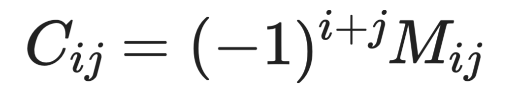
The cofactor

The (-1)^(i+j) term either keeps the minor's sign or flips it, depending on where you are in the matrix.

When i + j is even, (-1)^(i+j) = +1, so the cofactor equals the minor. When i + j is odd, (-1)^(i+j) = -1, so the cofactor flips the minor's sign.

The checkerboard pattern

This sign alternation creates a checkerboard pattern across the matrix:

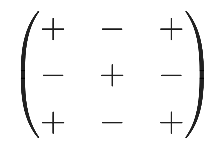
The checkerboard pattern

The top-left corner always starts with +. From there, signs alternate in every direction. This pattern tells you at a glance whether a cofactor will add or subtract from your determinant.

The Cofactor Expansion Formula

Here's the formula you’ve been waiting for.

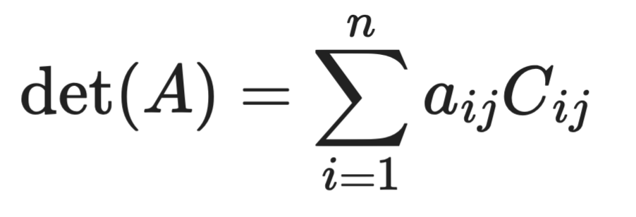
For expansion along row i:

Expansion along row i

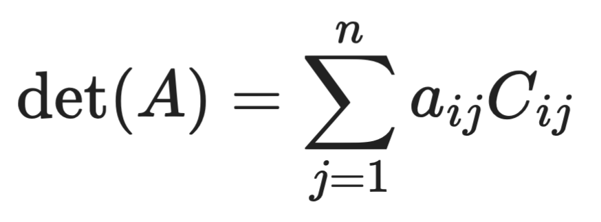
For expansion along column j:

Expansion along column j

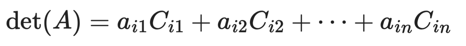
In plain English this means that you multiply each element in your chosen row or column by its cofactor, then add everything up.

The a_ij terms are just the individual elements of your matrix. The C_ij terms are the cofactors you compute for each position. Multiply them together, sum the results, and you've got your determinant.

It doesn't matter which row or column you pick. Expansion along row 1 gives the same result as expansion along row 3 or column 2. The determinant is a fixed property of the matrix - the expansion path is just your choice.

That choice does affect how much work you do, though. A row or column with more zeros means fewer cofactors to compute. If one row has two zeros and three non-zero elements, you only need to compute cofactors for those three elements - the zeros contribute nothing to the sum. Always scan your matrix for zeros before picking your expansion row or column.

Step-by-Step: How Cofactor Expansion Works

Cofactor expansion follows the same 3 step process every time.

Step 1: Choose a row or column. Scan your matrix and pick the row or column with the most zeros. Fewer non-zero elements means fewer cofactors to compute.

Step 2: For each non-zero element in that row or column:

• Compute the minor M_ij - delete row i and column j, then take the determinant of what's left.

• Apply the sign factor (-1)^(i+j) using the checkerboard pattern to get the cofactor C_ij.

• Multiply the element a_ij by its cofactor C_ij.

Step 3: Sum all the products.

The determinant

That's your determinant.

If any of your sub-matrices are larger than 2×2, repeat the same process on them until you're down to 2×2 determinants - which you can solve directly with ad - bc.

Example 1: Cofactor Expansion of a 2×2 Matrix

Let's connect everything with the simplest possible case.

Take this 2×2 matrix:

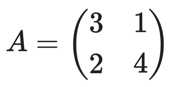
Sample 2x2 matrix

Expand along row 1. The two elements are a_11 = 3 and a_12 = 1.

• For a_11 = 3: delete row 1 and column 1. What's left is just (4). The sign factor is (-1)^(1+1) = +1. So C_11 = +4.

• For a_12 = 1: delete row 1 and column 2. What's left is just (2). The sign factor is (-1)^(1+2) = -1. So C_12 = -2.

Now sum the products:

Determinant calculation

You'll notice this matches the standard 2×2 formula ad - bc = (3)(4) - (1)(2) = 10. Cofactor expansion and the cross-multiplication shortcut are two ways to get the same answer.

Example 2: Cofactor Expansion of a 3×3 Matrix

Now let's work through a full 3×3 example.

Take this matrix:

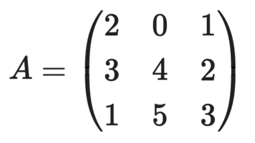
Sample 3x3 matrix

Row 1 has a zero in position (1,2), so let's expand along row 1. That zero means we can entirely skip one cofactor.

Step 1: Set up the expansion

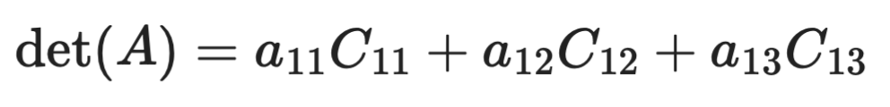
Expansion setup (1)

Since a_12 = 0, the middle term drops out:

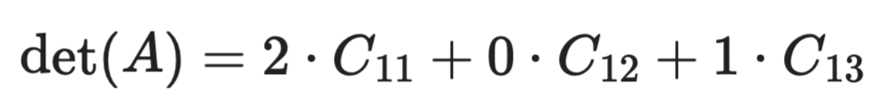
Expansion setup (2)

We only need to compute two cofactors. That's the payoff for choosing the right row.

Step 2: Compute C_11

Now delete row 1 and column 1. Here’s what's left:

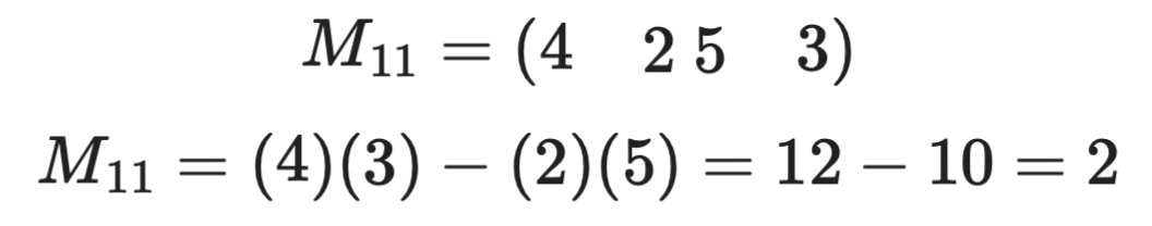
First computation

The sign at position (1,1) is (-1)^(1+1) = +1, so C_11 = +2.

Step 3: Compute C_13

The next step is to delete row 1 and column 3. This is left:

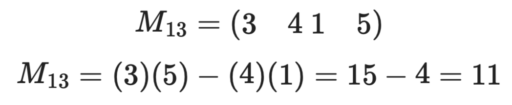
Second computation

The sign at position (1,3) is (-1)^(1+3) = +1, so C_13 = +11.

Step 4: Sum the products

Determinant calculation

That's your determinant. By picking the row with a zero upfront, you turned a three-cofactor problem into a two-cofactor one. Always work smarter.

Choosing the Best Row or Column

The row or column you pick doesn't change the result, but it does change how much work you do.

Always look for zeros first. Every zero in your chosen row or column is a cofactor you don't have to compute. In the 3×3 example above, one zero cut the work from three cofactors down to two. In larger matrices, a row with multiple zeros can save you from computing several sub-determinants.

Here’s a few points worth remembering

• One zero in a row or column means one fewer cofactor to compute
• Two zeros means two fewer cofactors
• All zeros except one means you only compute a single cofactor

This matters more as your matrix grows. A naive cofactor expansion on an n×n matrix runs in factorial time - meaning a 4×4 requires computing determinants of four 3×3 matrices, each of which expands into three 2×2 matrices. That's 24 individual calculations before you even start adding. For a 5×5, it's 120.

For large matrices, cofactor expansion isn't the right tool. Row reduction and LU decomposition handle big matrices much faster. Cofactor expansion is best kept for 2×2 and 3×3 cases, or for theoretical work where you need to symbolically express the determinant.

For anything you're solving by hand, spend a few seconds scanning for the row or column with the most zeros before you start. It's the simplest way to reduce arithmetic errors.

Cofactor Expansion and Recursive Structure

Cofactor expansion has a recursive structure built in.

To find the determinant of an n×n matrix, you expand along a row or column and compute determinants of (n-1)×(n-1) matrices. Each of those expands into (n-2)×(n-2) matrices. You keep reducing until you hit 2×2 matrices, which you solve directly.

This recursive property is what defines the determinant algebraically. It tells you what a determinant is at every matrix size, not just how to compute one.

Recursion has a cost, though.

Each level of expansion multiplies the number of sub-problems, and for large matrices the computation grows fast. That's why numerical libraries don't use cofactor expansion under the hood. Row reduction and factorization methods scale much better.

For small matrices and theoretical work, the recursive structure is exactly what you want. For anything larger, it’s better to look for another approach.

Connection to the Adjugate Matrix

Cofactors are the building block of matrix inversion. They’re not used just to help you compute determinants.

If you compute the cofactor C_ij for every element in a matrix A, you get a cofactor matrix C. Take the transpose of that - flip rows and columns - and you've got the adjugate matrix:

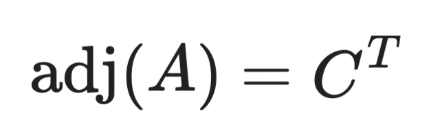
The adjugate matrix

From there, the matrix inverse follows directly:

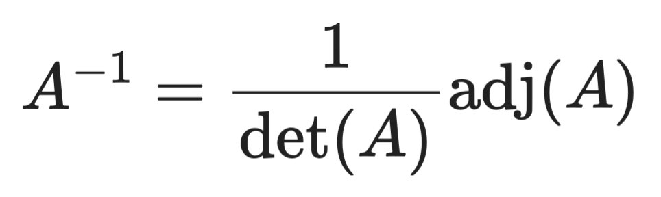
Matrix inverse

In plain terms this means you have to compute all the cofactors, arrange them into a matrix, transpose it, then divide by the determinant. That's your inverse.

There are two things worth remembering here:

1. This only works when det(A) ≠ 0 - a zero determinant means the matrix has no inverse
2. This formula is exact, which makes it useful for theoretical work and symbolic algebra. For numerical computation with large matrices, other methods are faster.

If you’re wondering about the connection with cofactor expansion, just remember that every entry in the adjugate matrix comes from a cofactor you'd compute during expansion. The same process that gives you the determinant also gives you everything you need to invert the matrix.

Properties of Cofactor Expansion

Cofactor expansion comes with a few properties worth knowing. They'll save you from second-guessing your work and help you spot shortcuts.

Here are four properties to remember:

• Expansion along any row or column gives the same result. You can expand along row 2 or column 3 - the determinant doesn't change. Pick whichever has the most zeros
• The determinant is linear in each row. If you scale a row by a constant k, the determinant scales by k too. This follows directly from how cofactors multiply into each element
• Swapping two rows flips the sign of the determinant. Swap rows once and the determinant negates. Swap twice and it's back to the original. This is why you need to carefully track row operations
• If two rows are linearly dependent, the determinant is zero. Linear dependence means one row is a scalar multiple of another - or more generally, that the rows don't span the full space. The matrix is singular, and no inverse exists

These properties are what lets you simplify matrices before expanding - reducing rows, spotting dependencies, and avoiding unnecessary computation.

Common Mistakes

Cofactor expansion has a few failure points that show up again and again. Here's what to watch for.

• Forgetting the (-1)^(i+j) sign. This is the most common mistake. You compute the minor correctly, multiply by the element, and get the wrong answer because you skipped the sign factor. Always check the checkerboard pattern before writing down a cofactor
• Deleting the wrong row or column for the minor. When computing M_ij, you delete row i and column j - the row and column of the element you're expanding on. A common slip is deleting the wrong one, especially in a 3×3 where the remaining matrix can look similar across different deletions
• Stopping too early in the recursion. When your sub-matrix is still 3×3 or larger, you need to expand again. Some people treat a 3×3 minor as if it were a 2×2 and apply ad - bc directly
• Arithmetic errors in recursive steps. The deeper the recursion, the more multiplications and sign flips you're tracking. A single arithmetic error in an early sub-determinant carries through every step that follows. Work through each 2×2 determinant carefully before combining results

If your final answer looks off, the sign pattern and the minor deletion are the first two things to recheck.

When to Use Cofactor Expansion

Cofactor expansion is the right tool in a few specific situations.

For small matrices, it's the most direct approach. A 2×2 is trivial, and a 3×3 is manageable by hand in a couple of minutes. Once you get to 4×4 and beyond, the number of recursive steps grows fast enough that other methods are faster and less error-prone.

It's also the go-to for theoretical and symbolic work. If you're working through a proof, deriving a formula, or computing a determinant with variable entries rather than numbers, cofactor expansion gives you an exact symbolic expression to work with. Row reduction is great for numbers, but it gets messy with symbols.

Here's a quick summary of when to reach for it:

• You're working with a 2×2 or 3×3 matrix
• You need an exact symbolic result, not a numerical approximation
• You're working through a proof that requires expanding the determinant explicitly
• You're building intuition for what the determinant actually means

For large numerical matrices, skip it. Row reduction and LU decomposition handle those cases much faster and with far less risk of compounding arithmetic errors. Most numerical libraries use these methods under the hood for exactly that reason.

Cofactor expansion is best thought of as a hand-calculation and theory tool, not a general-purpose algorithm.

Conclusion

Cofactor expansion gives you a systematic, recursive way to compute the determinant of any square matrix.

The two building blocks - minors and the (-1)^(i+j) sign pattern - drive the whole process. Get those right, and the rest is easy. Choose a row or column with zeros to cut down the work, reduce to 2×2 determinants, and sum the results.

Beyond determinants, the method connects to the adjugate matrix and the matrix inverse formula. The cofactors you compute during expansion are the same ones that build adj(A) - making cofactor expansion a foundation for understanding how matrix inversion works algebraically.

For small matrices and theoretical work, it's the most transparent method available. For large numerical matrices, you should go with row reduction or a numerical library.

If you want to see cofactor expansion in action, enroll in our Linear Algebra for Data Science in R course.