Course
Introduction to Python
4 hr
6.9M
This tutorial will walk you through some basic concepts and steps for data preparation. Data preparation is the first step after you get your hands on any kind of dataset. This is the step when you pre-process raw data into a form that can be easily and accurately analyzed. Proper data preparation allows for efficient analysis - it can eliminate errors and inaccuracies that could have occurred during the data gathering process and can thus help in removing some bias resulting from poor data quality. Therefore a lot of an analyst's time is spent on this vital step.
Loading data, cleaning data (removing unnecessary data or erroneous data), transforming data formats, and rearranging data are the various steps involved in the data preparation step. In this tutorial, you will work with Python's Pandas library for data preparation.
Make sure you understand concepts like Pandas DataFrame, Series, etc. since you will be reading about it a lot in this tutorial. You can learn more in-depth about pandas in DataCamp's Pandas tutorial.
In this tutorial:
On the way, there are some tips, tricks, and also reference to other in-depth material in case you want to dive deeper into a topic.
Let's start with a short introduction to Pandas...
Pandas is a software library written for Python. It is very famous in the data science community because it offers powerful, expressive, and flexible data structures that make data manipulation, analysis easy AND it is freely available. Furthermore, if you have a specific and new use case, you can even share it on one of the Python mailing lists or on pandas GitHub site - in fact, this is how most of the functionalities in pandas have been driven, by real-world use cases.
For an excellent introduction to pandas, be sure to check out DataCamp's Pandas Foundation course. It is very interactive, and the first chapter is free!
To use the pandas library, you need to first import it. Just type this in your python console:
import pandas as pdThe first step for data preparation is to... well, get some data. If you have a .csv file, you can easily load it up in your system using the .read_csv() function in pandas. You can then type:
data = pd.read_csv('path_to_file.csv')
However, for this tutorial, you shall be working with some smaller, easy-to-understand DataFrames and Series created on the fly.
This is a widespread problem in the data analysis world.
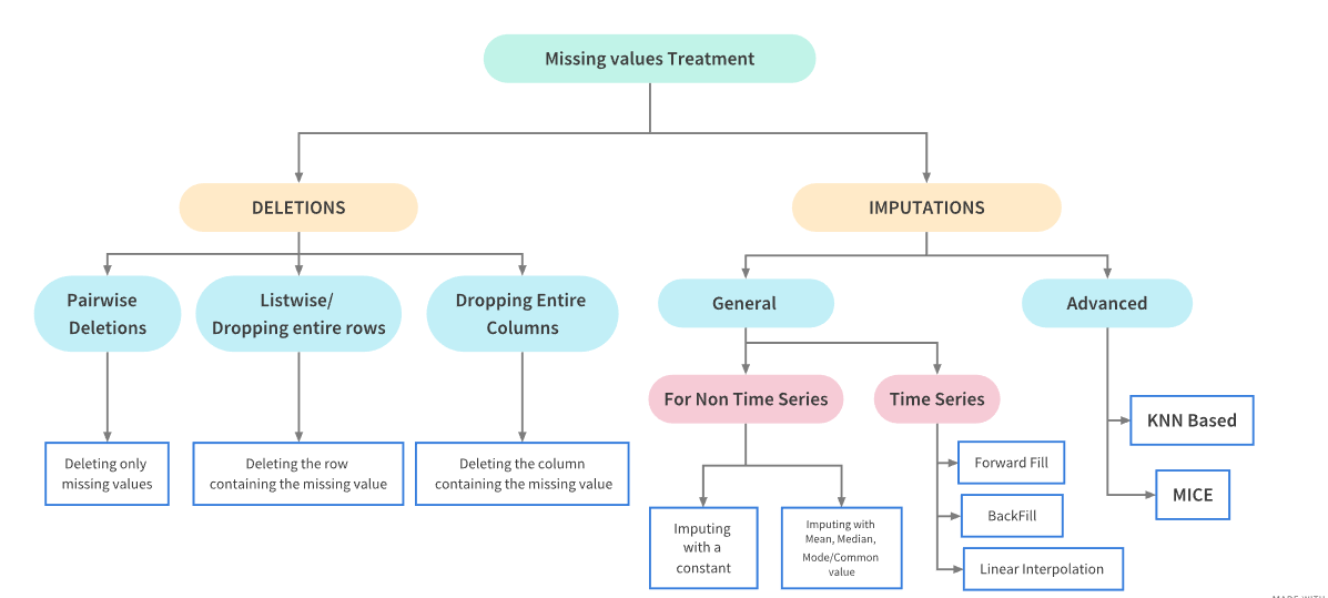
Missing data can arise in the dataset due to multiple reasons: the data for the specific field was not added by the user/data collection application, data was lost while transferring manually, a programming error, etc. It is sometimes essential to understand the cause because this will influence how you deal with such data. But this is coming up later on in this tutorial. For now, let's focus on what to do if you have missing data...
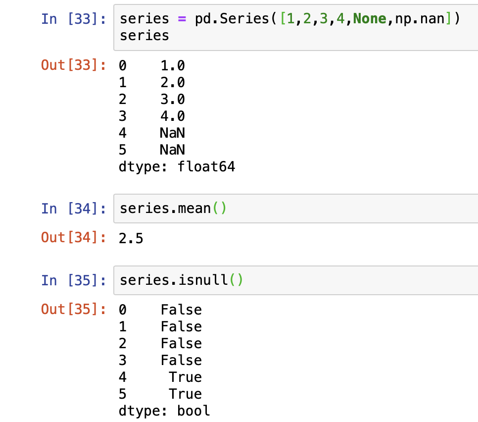
For numerical data, pandas uses a floating point value NaN (Not a Number) to represent missing data. It is a unique value defined under the library Numpy so we will need to import it as well. NaN is the default missing value marker for reasons of computational speed and convenience. This is a sentinel value, in the sense that it is a dummy data or flag value that can be easily detected and worked with using functions in pandas.
Let's play with some data...
import numpy as np

# Creating a pandas series
data = pd.Series([0, 1, 2, 3, 4, 5, np.nan, 6, 7, 8])

# To check if and what index in the dataset contains null value
data.isnull()
0    False
1    False
2    False
3    False
4    False
5    False
6     True
7    False
8    False
9    False
dtype: bool
Above, we used the function isnull() which returns a boolean true or false value. True, when the data at that particular index is actually missing or NaN. The opposite of this is the notnull() function.
# To check where the dataset does not contain null value - opposite of isnull()
data.notnull()
0     True
1     True
2     True
3     True
4     True
5     True
6    False
7     True
8     True
9     True
dtype: bool
Furthermore, we can use the dropna() function to filter out missing data and to remove the null (missing) value and see only the non-null values. However, the NaN value is not really deleted and can still be found in the original dataset.
# Will not show the index 6 cause it contains null (NaN) value
data.dropna()
0    0.0
1    1.0
2    2.0
3    3.0
4    4.0
5    5.0
7    6.0
8    7.0
9    8.0
dtype: float64
data
0    0.0
1    1.0
2    2.0
3    3.0
4    4.0
5    5.0
6    NaN
7    6.0
8    7.0
9    8.0
dtype: float64
What you can do to really "drop" or delete the NaN value is either store the new dataset (without NaN) so that the original data Series is not tampered or apply a drop inplace. The inplace argument has a default value of false.
not_null_data = data.dropna()
not_null_data
0    0.0
1    1.0
2    2.0
3    3.0
4    4.0
5    5.0
7    6.0
8    7.0
9    8.0
dtype: float64
# Drop the 6th index in the original 'data' since it has a NaN place
data.dropna(inplace = True)
data
0    0.0
1    1.0
2    2.0
3    3.0
4    4.0
5    5.0
7    6.0
8    7.0
9    8.0
dtype: float64
However, dataframes can be more complex and be 2 dimensions, meaning they contain rows and columns. Pandas still has you covered...
# Creating a dataframe with 4 rows and 4 columns (4*4 matrix)
data_dim = pd.DataFrame([[1,2,3,np.nan],[4,5,np.nan,np.nan],[7,np.nan,np.nan,np.nan],[np.nan,np.nan,np.nan,np.nan]])
data_dim
| 0 | 1 | 2 | 3 | |
|---|---|---|---|---|
| 0 | 1.0 | 2.0 | 3.0 | NaN |
| 1 | 4.0 | 5.0 | NaN | NaN |
| 2 | 7.0 | NaN | NaN | NaN |
| 3 | NaN | NaN | NaN | NaN |
Now let's say you only want to drop rows or columns that are all null or only those that contain a certain amount of null values. Check out the various scenarios, remember that the drop is not happening inplace, so the real dataset is not tampered. Pay attention to the arguments passed to the dropna() function to determine how you drop the missing data.
# Drop all rows and columns containing NaN value
data_dim.dropna()
| 0 | 1 | 2 | 3 |
|---|
# Drop all rows and columns containing entirely of NaN value
data_dim.dropna(how = 'all')
| 0 | 1 | 2 | 3 | |
|---|---|---|---|---|
| 0 | 1.0 | 2.0 | 3.0 | NaN |
| 1 | 4.0 | 5.0 | NaN | NaN |
| 2 | 7.0 | NaN | NaN | NaN |
# Drop only columns that contain entirely NaN value
# Default is 0 - which signifies rows
data_dim.dropna(axis = 1, how = 'all')
| 0 | 1 | 2 | |
|---|---|---|---|
| 0 | 1.0 | 2.0 | 3.0 |
| 1 | 4.0 | 5.0 | NaN |
| 2 | 7.0 | NaN | NaN |
| 3 | NaN | NaN | NaN |
# Drop all columns that have more than 2 NaN values
data_dim.dropna(axis = 1, thresh = 2)
| 0 | 1 | |
|---|---|---|
| 0 | 1.0 | 2.0 |
| 1 | 4.0 | 5.0 |
| 2 | 7.0 | NaN |
| 3 | NaN | NaN |
# Drop all rows that have more than 2 NaN values
data_dim.dropna(thresh = 2)
| 0 | 1 | 2 | 3 | |
|---|---|---|---|---|
| 0 | 1.0 | 2.0 | 3.0 | NaN |
| 1 | 4.0 | 5.0 | NaN | NaN |
Now you know how to identify and drop missing values - whether to simply see the resultant dataset or do an inplace deletion. In many cases, simply dropping the null values is not a feasible option, and you might want to fill in the missing data with some other value. Let's see how you can do that...
To replace or rather "fill in" the null data, you can use the fillna() function. For example, let's try to use the same dataset as above and try to fill in the NaN values with 0.
# Check what the dataset looks like again
data_dim
| 0 | 1 | 2 | 3 | |
|---|---|---|---|---|
| 0 | 1.0 | 2.0 | 3.0 | NaN |
| 1 | 4.0 | 5.0 | NaN | NaN |
| 2 | 7.0 | NaN | NaN | NaN |
| 3 | NaN | NaN | NaN | NaN |
# Fill the NaN values with 0
data_dim_fill = data_dim.fillna(0)
data_dim_fill
| 0 | 1 | 2 | 3 | |
|---|---|---|---|---|
| 0 | 1.0 | 2.0 | 3.0 | 0.0 |
| 1 | 4.0 | 5.0 | 0.0 | 0.0 |
| 2 | 7.0 | 0.0 | 0.0 | 0.0 |
| 3 | 0.0 | 0.0 | 0.0 | 0.0 |
And like with dropna() you can also do many other things depending on the kind of argument you pass. Also a reminder that passing the inplace = True argument will make the change to the original dataset.
# Pass a dictionary to use differnt values for each column
data_dim_fill = data_dim.fillna({0: 0, 1: 8, 2: 9, 3: 10})
data_dim_fill
| 0 | 1 | 2 | 3 | |
|---|---|---|---|---|
| 0 | 1.0 | 2.0 | 3.0 | 10.0 |
| 1 | 4.0 | 5.0 | 9.0 | 10.0 |
| 2 | 7.0 | 8.0 | 9.0 | 10.0 |
| 3 | 0.0 | 8.0 | 9.0 | 10.0 |
You can pass a method argument to the fillna() function that automatically propogates non-null values forward (ffill or pad) or backward (bfill or backfill).
# Pass method to determine how to fill-up the column - forward here
data_dim_fill = data_dim.fillna(method='ffill')
data_dim_fill
| 0 | 1 | 2 | 3 | |
|---|---|---|---|---|
| 0 | 1.0 | 2.0 | 3.0 | NaN |
| 1 | 4.0 | 5.0 | 3.0 | NaN |
| 2 | 7.0 | 5.0 | 3.0 | NaN |
| 3 | 7.0 | 5.0 | 3.0 | NaN |
You can also limit the number of fills above. For example, fill up only two places in the columns... Also, if you pass axis = 1 this will fill out row value accordingly.
# Pass method to determine how to fill-up the column - forward here
data_dim_fill = data_dim.fillna(method='ffill', limit = 2)
data_dim_fill
| 0 | 1 | 2 | 3 | |
|---|---|---|---|---|
| 0 | 1.0 | 2.0 | 3.0 | NaN |
| 1 | 4.0 | 5.0 | 3.0 | NaN |
| 2 | 7.0 | 5.0 | 3.0 | NaN |
| 3 | 7.0 | 5.0 | NaN | NaN |
# Pass method to determine how to fill-up the row - forward here
data_dim_fill = data_dim.fillna(axis = 1, method='ffill')
data_dim_fill
| 0 | 1 | 2 | 3 | |
|---|---|---|---|---|
| 0 | 1.0 | 2.0 | 3.0 | 3.0 |
| 1 | 4.0 | 5.0 | 5.0 | 5.0 |
| 2 | 7.0 | 7.0 | 7.0 | 7.0 |
| 3 | NaN | NaN | NaN | NaN |
With some understanding of the data and your use-case, you can use the fillna() function in many other ways than simply filling it with numbers. You could fill it up using the mean using the mean() or the median value median() as well...
# Check the data_dim dataset
data_dim
| 0 | 1 | 2 | 3 | |
|---|---|---|---|---|
| 0 | 1.0 | 2.0 | 3.0 | NaN |
| 1 | 4.0 | 5.0 | NaN | NaN |
| 2 | 7.0 | NaN | NaN | NaN |
| 3 | NaN | NaN | NaN | NaN |
# Fill the NaN value with mean values in the corresponding column
data_dim_fill = data_dim.fillna(data_dim.mean())
data_dim_fill
| 0 | 1 | 2 | 3 | |
|---|---|---|---|---|
| 0 | 1.0 | 2.0 | 3.0 | NaN |
| 1 | 4.0 | 5.0 | 3.0 | NaN |
| 2 | 7.0 | 3.5 | 3.0 | NaN |
| 3 | 4.0 | 3.5 | 3.0 | NaN |
So far, you have only worked with missing data (NaN), but there could be situations where you would want to replace a non-null value with a different value. Or maybe a null value is recorded as a random number, and hence needs to be processed as NaN rather than a number. This is where the replace() function comes in handy...
Let's create a different dataset this time.
data = pd.Series([1,2,-99,4,5,-99,7,8,-99])
data
0     1
1     2
2   -99
3     4
4     5
5   -99
6     7
7     8
8   -99
dtype: int64
# Replace the placeholder -99 as NaN
data.replace(-99, np.nan)
0    0.0
1    1.0
2    2.0
3    3.0
4    4.0
5    5.0
7    6.0
8    7.0
9    8.0
dtype: float64
You will no longer see the -99, because it is replaced by NaN and hence not shown. Similarly, you can pass multiple values to be replaced. To do this, we will create another series and then concatenate the original data series with the new series and then apply the multiple value replace function.
To do this, we can use the concat() function in pandas. To continue the indexing after applying the concatenation, you can pass the ignore_index = True argument to it.
# Create a new Series
new_data = pd.Series([-100, 11, 12, 13])
combined_series = pd.concat([data, new_data], ignore_index = True)
combined_series
0       1
1       2
2     -99
3       4
4       5
5     -99
6       7
7       8
8     -99
9    -100
10     11
11     12
12     13
dtype: int64
# Let's replace -99 and -100 as NaN in the new combined_series
data_replaced = combined_series.replace([-99, -100], np.nan)
data_replaced
0      1.0
1      2.0
2      NaN
3      4.0
4      5.0
5      NaN
6      7.0
7      8.0
8      NaN
9      NaN
10    11.0
11    12.0
12    13.0
dtype: float64
# Argument passed can also be a dictionary with separate values
data_replaced = combined_series.replace({-99: np.nan, -100: 0})

# Same as: new_data.replace([-99, -100], [np.nan, 0])
data_replaced
0      1.0
1      2.0
2      NaN
3      4.0
4      5.0
5      NaN
6      7.0
7      8.0
8      NaN
9      0.0
10    11.0
11    12.0
12    13.0
dtype: float64
In some situations, you might want to add more insight to what you already have based on some logic. This is when you can take help from maps and a combination of functions to achieve what you want. The logic can get more complicated, but try understanding with the help of this example.
Let's say, you have a dataframe of numbers mapped to its corresponding count in English.
data_number = pd.DataFrame({'english': ['zero','one','two','three','four','five'],
'digits': [0,1,2,3,4,5]})
data_number
| english | digits | |
|---|---|---|
| 0 | zero | 0 |
| 1 | one | 1 |
| 2 | two | 2 |
| 3 | three | 3 |
| 4 | four | 4 |
| 5 | five | 5 |
Let's say you now want to add another column indicating multiples of two as 'Yes' and the rest as 'No'. You can write down a mapping of each distinct English calls to it's corresponding 'Yes' or 'No'.
english_to_multiple = {
    'two': 'yes',
    'four': 'yes'
}
Then you can call the map function to add the column for when the English column is a multiple of 2. What gets filled in the other non-multiple number columns? Let's find out...
data_number['multiple'] = data_number['english'].map(english_to_multiple)
data_number
| english | digits | multiple | |
|---|---|---|---|
| 0 | zero | 0 | NaN |
| 1 | one | 1 | NaN |
| 2 | two | 2 | yes |
| 3 | three | 3 | NaN |
| 4 | four | 4 | yes |
| 5 | five | 5 | NaN |
The other columns are filled with NaN values, and you already know how to further work with missing values. This was a simple example. But hope you can find inspiration to use ideas from here to use the map function to do more stuff and utilize it in your specific use-cases.
Sometimes you might want to categorize based on some logic and put all the data into discrete buckets or bins for analysis purpose. You can use the cut() function for this. For example, let's first create a dataset containing 30 random numbers between 1 - 100.
import random

data = random.sample(range(1, 101), 30)
# data
[45,
 39,
 25,
 83,
 27,
 6,
 73,
 43,
 36,
 93,
 97,
 17,
 15,
 99,
 37,
 5,
 31,
 22,
 65,
 30,
 3,
 26,
 91,
 12,
 52,
 76,
 63,
 84,
 59,
 53]
Say we want to categorize those in terms of some bucket we define ourselves: numbers between 1 - 25, then 25 - 35, 40 - 60 and then 60 - 80 and then the rest. So we define a bucket...
Then we will use the cut function.
# Defining the starting value for each bucket
bucket = [1, 25, 35, 60, 80, 100]

cut_data = pd.cut(data, bucket)
cut_data
[(35, 60], (35, 60], (1, 25], (80, 100], (25, 35], ..., (60, 80], (60, 80], (80, 100], (35, 60], (35, 60]]
Length: 30
Categories (5, interval[int64]): [(1, 25] < (25, 35] < (35, 60] < (60, 80] < (80, 100]]
cut() is a very useful function, and there is much more you can do with it. It is highly recommended that you check out the Pandas document to learn more about it.
This topic is particularly useful when you want to be able to convert some categorical data into numerical values so that you can use it in your data analysis model. This is particularly handy, especially when doing machine learning modeling, where the concept of one-hot encoding is famous. Using more technical words: one-hot encoding is the process of converting categorical values into a 1-dimensional numerical vector.
One way of doing this using pandas is to use the get_dummies() function. If a column in your dataframe has 'n' distinct values, the function will derive a matrix with 'n' columns containing all 1s and 0s. Let's see this with an example to grasp the concept better...
# Creating a DataFrame consiting individual characters in the list
data = pd.Series(list('abcdababcdabcd'))
data
0     a
1     b
2     c
3     d
4     a
5     b
6     a
7     b
8     c
9     d
10    a
11    b
12    c
13    d
dtype: object
Let's say now you want to have individual vectors indicating the appearance of each character to feed it to a function.
Something like this: for 'a' = [1,0,0,0,1,0,1,0,0,0,1,0,0,0] where 1 is in the position where 'a' exists and 0 for where it does not. Using the get_dummies() function will make the task easier.
pd.get_dummies(data)
| a | b | c | d | |
|---|---|---|---|---|
| 0 | 1 | 0 | 0 | 0 |
| 1 | 0 | 1 | 0 | 0 |
| 2 | 0 | 0 | 1 | 0 |
| 3 | 0 | 0 | 0 | 1 |
| 4 | 1 | 0 | 0 | 0 |
| 5 | 0 | 1 | 0 | 0 |
| 6 | 1 | 0 | 0 | 0 |
| 7 | 0 | 1 | 0 | 0 |
| 8 | 0 | 0 | 1 | 0 |
| 9 | 0 | 0 | 0 | 1 |
| 10 | 1 | 0 | 0 | 0 |
| 11 | 0 | 1 | 0 | 0 |
| 12 | 0 | 0 | 1 | 0 |
| 13 | 0 | 0 | 0 | 1 |
However, this is a simple example to help you get started. In real world applications the membership of a character can belong to various categories at the same time, thus you will have to learn more sophisticated methods. Also for much larger data, this function might not be very efficient in terms of speed. DataCamp's Handling Categorical Data in Python discusses such cases and the topic more in-depth.
Well, you are at the end of the tutorial, and you have learned some basic tools to start the first step in your data analysis path. Other skills to learn for the data preparation steps would also be to learn how to detect and filter outliers in your dataset and if the dataset is vast - maybe start with random sampling. But these are again broad topics in themselves and hard to generalize.
Real world use cases can often be more complex and might need its own unique solution, but the idea is to start small and learn on the way and to explore more and get your hands dirty with different datasets! Be sure to check out DataCamp's Cleaning Data in Python course to learn more tools and tricks and in the end, you get to work on a real-world, messy dataset obtained from the Gapminder Foundation. Go get started!
Python Courses
Course
Course
Course
cheat-sheet
Karlijn Willems
Tutorial
DataCamp Team
Tutorial
Kurtis Pykes
Tutorial
Karlijn Willems
Tutorial
Vidhi Chugh
Tutorial
DataCamp Team