Detect Anomalies with Anomalize in R

Anaomalize: Brief Description

When we talk about anomalies, we consider the data points that are outliers or an exceptional event. Identifying those events are easy in small data sets and can be done with some simple analysis graphs like boxplots. But the cases will simultaneously get complicated when switched to large data sets, especially in the case of time series. Time series is the data captured on a fixed interval of time over a time period, when analyzed shows a trend or seasonality. Identifying anomalies in these cases is kind of a tricky aspect.

Then comes the anomalize package for anomaly detection in time series analysis, it's a tidy anomaly detection algorithm that’s time-based and scalable from one to many time series.

There are some available packages and methods that help in its development, or you can say that its a combination of available resources with a scalable approach.

The open source work that helped are as follow:

• Twitter’s AnomalyDetection package: Available on Github(cran anaomalyDetection is a different work).
• Rob Hyndman’s forecast::tsoutliers() function available through forecast package.
• Javier Lopez-de-lacalle’s package, tsoutliers, on CRAN.

These all packages and functions are used to integrate into a scalable workflow.

Talking about the workflow of anomalize, it is divided into three parts:

• Time series decomposition with time_decompose().
• Anomaly detection of remainder with anomalize().
• Anomaly lower and upper bound transformation with time_recompose().

Workflow of Anomaly detection

Time Series Decomposition

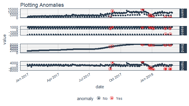
The first step is the time series decomposition using time_decompose(). The measured value or the numerical value on which detection needs to be performed for a particular group is decomposed into four columns that are observed, season, trend, and remainder. The default method used for decomposition is stl, which is a seasonal decomposition utilizing a Loess smoother.

Loess regression is the most common method used to smoothen a volatile time series, it fits multiple regression in local neighborhood, you can also say that the data is divided and regression is applied to each part, which is useful in time series because we know the bound of time which is the X variable in this case. This method works well in the case where the trend dominates the seasonality of the time series.

Here trend is long-term growth that happens over many observations and seasonality is the cyclic pattern occurring on a daily cycle for a minute or an hour or weekly.

There is a second technique which you can use for seasonal decomposition in time series based on median that is the Twitter method which is also used AnomalyDetection package. It is identical to STL for removing the seasonal component. The difference is in removing the trend is that it uses piece-wise median of the data(one or several median split at specified intervals) rather than fitting a smoother. This method works well where seasonality dominates the trend in time series.

Let's talk about the output of the time_decompose() function, as discussed above it produces 4 columns:

• observed : The actual values.
• season : The seasonal or cyclic trend. The default is a weekly seasonality.
• trend : The long-term trend. The default is a span of 3 months.
• remainder : It is used for analyzing the outliers. It is merely the observed minus both the season and trend.

The time_decompose() function contains an argument merge, by setting it TRUE we can keep the original data along with the produced columns.

# Using data package provided in the anomalize package and taking single time series of package purrr

purrr_package = tidyverse_cran_downloads%>%
  filter(package == "purrr")%>%
  ungroup()

purrr_anomaly  = purrr_package %>%
  time_decompose(count)

purrr_anomaly%>% glimpse()

 ## Observations: 425
## Variables: 5
## $ date      <date> 2017-01-01, 2017-01-02, 2017-01-03, 2017-01-04, 201...
## $ observed  <dbl> 550, 1012, 1515, 1702, 1696, 1613, 860, 796, 2008, 2...
## $ season    <dbl> -2158.8893, 692.6571, 1087.5708, 1052.3294, 939.9377...
## $ trend     <dbl> 1496.712, 1511.009, 1525.307, 1539.604, 1553.901, 15...
## $ remainder <dbl> 1212.1777, -1191.6661, -1097.8773, -889.9334, -797.8...

Detecting anomalies in the remainders

After the time series analysis is complete and the remainder has the desired characteristics to perform anomaly detection which again creates three new columns.

• remainder_l1 : The lower limit of the remainder.
• remainder_l2 : The upper limit of the remainder.
• anaomaly : Column is telling whether the observation is an anomaly or not.

Anomalies are high leverage points that distort the distribution. The anomalize implements two methods that are resistant to high leverage points:

• IQR: Inner Quartile Range
• GESD: Generalized Extreme Studentized Deviate Test

IQR

It is a similar method used in tsoutliers() function of the forecast package. In IQR a distribution is taken and 25% and 75% inner quartile range to establish the distribution of the remainder. Limits are set by default to a factor of 3 times above, and below the inner quartile range, any remainder beyond the limit is considered as an anomaly.

GESD

In GESD anomalies are progressively evaluated removing the worst offenders and recalculating the test statistics and critical values, or more simply you can say that a range is recalculated after identifying the anomalies in an iterative way.

Both IQR and GESD have their Pros and cons, IQR is comparatively faster as there are no loops involved in the IQR but it's not as accurate as GESD since the anomalies skews the median which is removed in GESD.

purrr_anomaly = purrr_anomaly%>%
  anomalize(remainder)

purrr_anomaly%>% glimpse()

## Observations: 425
## Variables: 8
## $ date         <date> 2017-01-01, 2017-01-02, 2017-01-03, 2017-01-04, ...
## $ observed     <dbl> 550, 1012, 1515, 1702, 1696, 1613, 860, 796, 2008...
## $ season       <dbl> -2158.8893, 692.6571, 1087.5708, 1052.3294, 939.9...
## $ trend        <dbl> 1496.712, 1511.009, 1525.307, 1539.604, 1553.901,...
## $ remainder    <dbl> 1212.1777, -1191.6661, -1097.8773, -889.9334, -79...
## $ remainder_l1 <dbl> -4330.511, -4330.511, -4330.511, -4330.511, -4330...
## $ remainder_l2 <dbl> 4400.459, 4400.459, 4400.459, 4400.459, 4400.459,...
## $ anomaly      <chr> "No", "No", "No", "No", "No", "No", "No", "No", "...

Anomaly lower and upper bound transformation

The last step of the workflow is to create lower and upper bounds around the observed values with time_recompose. It recomposes the season, trend, remainder_l1 and remainder_l2 into new limits that are:

• recomposed_l1 : The lower bound of outliers around the observed values.
• recomposed_l2 : The upper bound of outliers around the observed values.

purrr_anomaly = purrr_anomaly%>%
  time_recompose()

purrr_anomaly%>% glimpse()

## Observations: 425
## Variables: 10
## $ date          <date> 2017-01-01, 2017-01-02, 2017-01-03, 2017-01-04,...
## $ observed      <dbl> 550, 1012, 1515, 1702, 1696, 1613, 860, 796, 200...
## $ season        <dbl> -2158.8893, 692.6571, 1087.5708, 1052.3294, 939....
## $ trend         <dbl> 1496.712, 1511.009, 1525.307, 1539.604, 1553.901...
## $ remainder     <dbl> 1212.1777, -1191.6661, -1097.8773, -889.9334, -7...
## $ remainder_l1  <dbl> -4330.511, -4330.511, -4330.511, -4330.511, -433...
## $ remainder_l2  <dbl> 4400.459, 4400.459, 4400.459, 4400.459, 4400.459...
## $ anomaly       <chr> "No", "No", "No", "No", "No", "No", "No", "No", ...
## $ recomposed_l1 <dbl> -4992.689, -2126.845, -1717.634, -1738.578, -183...
## $ recomposed_l2 <dbl> 3738.281, 6604.125, 7013.336, 6992.392, 6894.298...

Plotting Anomalies

purrr_anomaly%>%
  plot_anomaly_decomposition()+
  ggtitle("Plotting Anomalies")

Tuning parameters

Modeling an anomaly detector would be incomplete without adjusting the parameters which are entirely dependent on data.

Let's get into adjusting parameters, so the parameters of each level of the workflow are different as each level of the workflow is performing its own task.

Adjusting parameters of decomposition

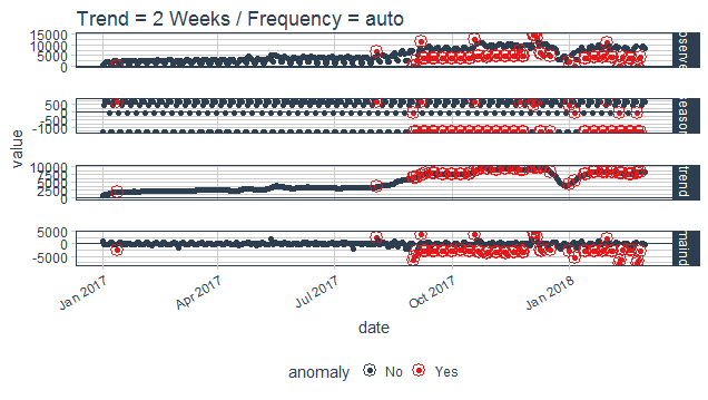
As discussed before the trend and seasonality are fundamentals for decomposing a time series, so adjustment should also be done in frequency and trend of the function time_decompose. By default, the values are auto-assigned which is 7 days for frequency in both methods (STL, Twitter), and for trend its 91 days for STL and 85 days for Twitter.

You can tweak both or single argument according to your comfort but look carefully before adjusting as changing without observation can overfit or underfit the decomposition process.

purrr_package %>%
  time_decompose(count, frequency = "auto", trend = "2 weeks")%>%
  anomalize(remainder)%>%
  plot_anomaly_decomposition()+
  ggtitle("Trend = 2 Weeks / Frequency = auto ")

Adjusting parameters for Anomaly detection

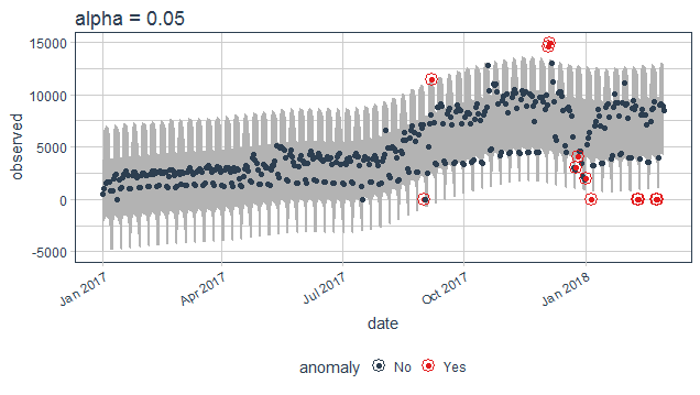
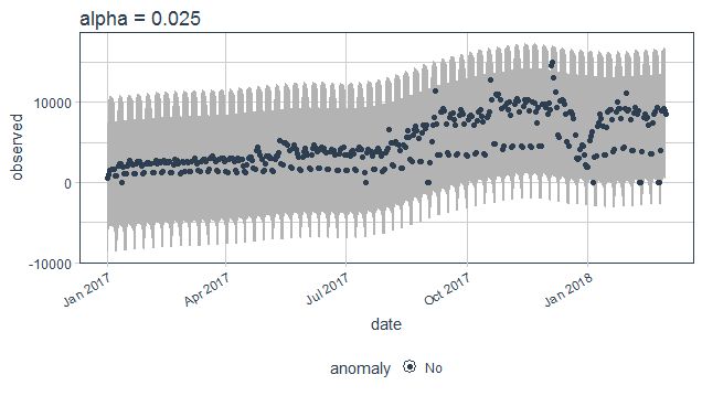
As discussed above here anomaly is being decided according to the values of remainder calculating limits for categorizing the outliers. The alpha and max_anoms are two parameters that control anomalize() function. In simple words alpha control the band of the limit by default it is set to 0.05 decreasing its value will increase the size of the band thus making difficult for a point to be an anomaly.

purrr_package%>%
  time_decompose(count)%>%
  anomalize(remainder, alpha = 0.05)%>%
  time_recompose()%>%
  plot_anomalies(time_recompose = T)+
  ggtitle("alpha = 0.05")

purrr_package%>%
  time_decompose(count)%>%
  anomalize(remainder, alpha = 0.025)%>%
  time_recompose()%>%
  plot_anomalies(time_recompose = T)+
  ggtitle("alpha = 0.025")

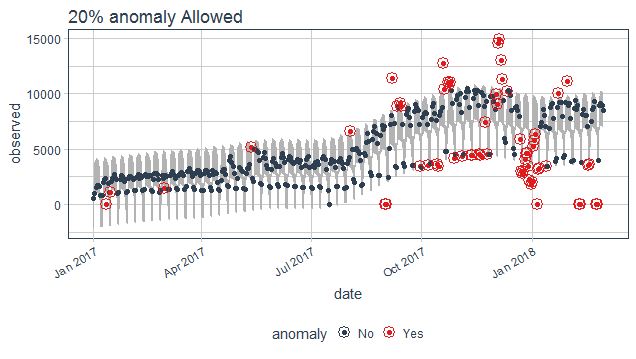
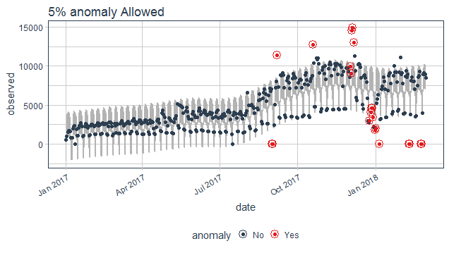
The max_anom parameter controls the percentage of data that can be an anomaly. This parameter is useful where alpha is too difficult to tune, and you want to focus on most aggressive anomalies.

purrr_package%>%
  time_decompose(count)%>%
  anomalize(remainder, alpha = 0.2, max_anoms = 0.2)%>%
  time_recompose()%>%
  plot_anomalies(time_recompose = T)+
  ggtitle("20% anomaly Allowed")

purrr_package%>%
  time_decompose(count)%>%
  anomalize(remainder, alpha = 0.2, max_anoms = 0.05)%>%
  time_recompose()%>%
  plot_anomalies(time_recompose = T)+
  ggtitle("5% anomaly Allowed")

References

• Anomalize all functions references in detail
• Interesting blog with all details

If you would like to learn more about R, take DataCamp's Introduction to Time Series Analysis course.

Check out our Time Series Analysis using R: Tutorial.