Course
Machine Learning with Tree-Based Models in Python
5 hr
116.4K
Consider the following situation -
You are working on your dataset. You create a classification model and get 90% accuracy immediately. The results seem fantastic to you. You dive a little deeper and discover that almost entirety of the data belongs to one class. Damn! Imbalanced data can cause you a lot of frustration.
You feel very frustrated when you discovered that your data has imbalanced classes and that all of the great results you thought you were getting turn out to be a lie. What is even more frustrating is the good books don't even holistically cover this topic.
This is an example of a situation cases by an imbalanced dataset and the frustrating results it can cause.
In this tutorial, you will discover the techniques that you can use to deliver excellent results on datasets with imbalanced data. Specifically, you will cover:
Let's first see what imbalanced data is.
 Source: KDNuggets
Imbalanced data typically refers to classification tasks where the classes are not represented equally.
For example, you may have a binary classification problem with 100 instances out of which 80 instances are labeled with Class-1, and the remaining 20 instances are marked with Class-2.
This is essentially an example of an imbalanced dataset, and the ratio of Class-1 to Class-2 instances is 4:1.
Be it a Kaggle competition or real test dataset, the class imbalance problem is one of the most common ones.
Most of the real-world classification problems display some level of class imbalance, which happens when there are not sufficient instances of the data that correspond to either of the class labels. Therefore, it is imperative to choose the evaluation metric of your model correctly. If it is not done, then you might end up adjusting/optimizing a useless parameter. In a real business-first scenario, this may lead to a complete waste.
There are problems where a class imbalance is not just common; it is bound to happen. For example, the datasets that deal with fraudulent and non-fraudulent transactions, it is very likely that the number of fraudulent transactions as compares to the number of non-fraudulent transactions will be very much less. And this is where the problem arises. You will study why.
Although all many machine learning algorithms (both deep and statistical) have shown great success in many real-world applications, the problem of learning from imbalanced data is still yet to be state-of-the-art. And often, this learning from imbalanced data is referred to as Imbalanced learning.
Following are the significant problems of imbalanced learning:
At this point of time one obvious question that must have come to your mind is - why in an age of GPUs, TPUs machine learning algorithms are failing to tackle imbalanced data efficiently? Quite an obvious question and you will find its answer now.
Evaluation of machine learning algorithms has a lot to do as to the reason why a particular machine learning algorithm does not perform when supplied with imbalanced data.
"It is the case where your accuracy measures tell the story that you have excellent accuracy (such as 90%), but the accuracy is only reflecting the underlying class distribution." - Machine Learning Mastery
Suppose, you have a dataset (associated with a classification task) with two classes with a distribution ratio of 9:1. The total number of instances present in the dataset is 1000, and the class labels are Class-1 and Class-2. Therefore, w.r.t the distribution ratio, the number of instances that correspond to Class-1 is 900 while Class-2 instances are 100. Now, you applied a standard classifier (say Logistic Regression) and measured its performance concerning classification accuracy which gives the number of instances correctly classified by the classifier. Now, take a closer look and think very deeply.
You Logistic Regression model does not have to be very complicated to classify all the 1000 instances as Class-1. In that case, you would get a classification accuracy of 90% which is really not enough to test the actual quality of the classifier. Clearly, you need some other metric to evaluate the performance of the system. You will see that in a minute. The phenomenon you just studied is called Accuracy Paradox.
You will start this section by studying some metrics other than classification accuracy in order to truly judge a classifier when it is dealing with imbalanced data.
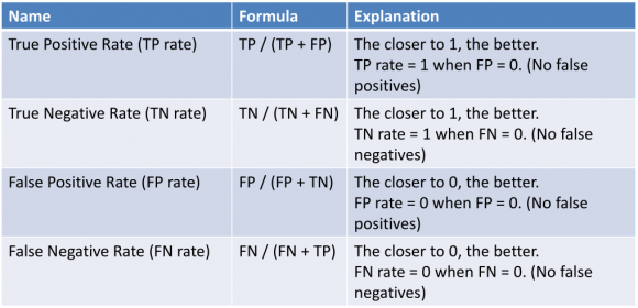
First, let's define four fundamental terms here:
The following image will justify the above terms for themselves:
Now, assume that you trained another classifier on the toy dataset you just saw and this time you applied a Random Forest. And you got a classification accuracy of 70%. Now that, you know about True Positive and Negative Rates and False Positive and Negative Rates, you will investigate the performance of the earlier Logistic Regression and Random Forest in a bit more detailed manner.
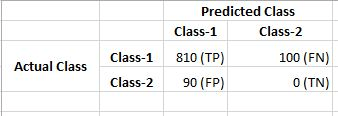
Suppose you got the following True Positive and Negative Rates and False Positive and Negative Rates for Logistic Regression:
Now, assume that the True Positive and Negative Rates and False Positive and Negative Rates for Random Forest are following:
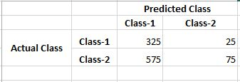
Just look at the number of negative classes correctly predicted (True Negatives) by both of the classifiers. As you are dealing with an imbalanced dataset, you need to give this number the most priority (because Class-1 dominant in the dataset). So, considering that, Random Forest trades away Logistic Regression easily.
Now, you are in an excellent place to study the approaches for combating imbalanced dataset problem.
(Remember, the above representation is popularly known as Confusion Matrix.)
Following are the two terms that are derived from the confusion matrix and very much used when you are evaluating a classifier.
Precision: Precision is the number of True Positives divided by the number of True Positives and False Positives. Put another way; it is the number of positive predictions divided by the total number of positive class values predicted. It is also called the Positive Predictive Value (PPV).
Precision can be thought of as a measure of a classifier's exactness. A low precision can also indicate a large number of False Positives.
Recall: Recall is the number of True Positives divided by the number of True Positives and the number of False Negatives. Put another way it is the number of positive predictions divided by the number of positive class values in the test data. It is also called Sensitivity or the True Positive Rate.
Recall can be thought of as a measure of a classifier's completeness. A low recall indicates many False Negatives.
Some other metrics that can be useful in this context:
Before, you begin studying the approaches to tackle class-imbalance problem let's take a very real-world example where just choosing classification accuracy as the evaluation metric can produce disastrous results. (You are doing this to ensure you do not only consider classification accuracy when you train your next classifier.)
The breast cancer dataset is a standard machine learning dataset. It contains 9 attributes describing 286 women that have suffered and survived breast cancer and whether or not breast cancer recurred within 5 years. Let's investigate this dataset to get you a real feel of the problem.
The dataset concerns a binary classification problem. Of the 286 women, 201 did not suffer a recurrence of breast cancer, leaving the remaining 85 that did.
Let's explore about the dataset more visually.
import numpy as np
import pandas as pd

# Load the dataset into a pandas dataframe
data = pd.read_csv("breast-cancer.data",header=None)

# See the data
print(data.head(10))
                      0      1        2      3    4   5  6      7          8  \
0  no-recurrence-events  30-39  premeno  30-34  0-2  no  3   left   left_low
1  no-recurrence-events  40-49  premeno  20-24  0-2  no  2  right   right_up
2  no-recurrence-events  40-49  premeno  20-24  0-2  no  2   left   left_low
3  no-recurrence-events  60-69     ge40  15-19  0-2  no  2  right    left_up
4  no-recurrence-events  40-49  premeno    0-4  0-2  no  2  right  right_low
5  no-recurrence-events  60-69     ge40  15-19  0-2  no  2   left   left_low
6  no-recurrence-events  50-59  premeno  25-29  0-2  no  2   left   left_low
7  no-recurrence-events  60-69     ge40  20-24  0-2  no  1   left   left_low
8  no-recurrence-events  40-49  premeno  50-54  0-2  no  2   left   left_low
9  no-recurrence-events  40-49  premeno  20-24  0-2  no  2  right    left_up

    9
0  no
1  no
2  no
3  no
4  no
5  no
6  no
7  no
8  no
9  no
The column names are numeric because you are using a partially preprocessed dataset. But if you are interested then you may refer to the following image:

Let's see a bar graph of the class distributions.
import matplotlib.pyplot as plt

classes = data[9].values
unique, counts = np.unique(classes, return_counts=True)

plt.bar(unique,counts)
plt.title('Class Frequency')
plt.xlabel('Class')
plt.ylabel('Frequency')
plt.show()
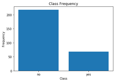
You can clearly see the class imbalance here. yes denotes the instances which have cancer and is obvious, the number of these instances is minimal as compared to the instances corresponding to the other class.
Let's define "No Recurrences" and "Recurrences" event that is there in the dataset which will make things even more evident.
All No Recurrence: A model that only predicted no recurrence of breast cancer would achieve an accuracy of (201/286) * 100 or 70.28%. This is called All No Recurrence. This is a high accuracy, but a terrible model. If this model was misinterpreted, it would send home 85 women incorrectly thinking their breast cancer was not going to reoccur (High False Negatives).
All recurrence: A model that only predicted the recurrence of breast cancer would achieve an accuracy of (85/286) * 100 or 29.72%. This is known All Recurrence. This model fails at producing good accuracy and would send home 201 women thinking that had a recurrence of breast cancer, but this is not the case (High False Positives).
This concept should have sparked an ignition inside you by now. Let's move forward with it.
Well! Now, you have now enough reasons to wonder why considering only classification accuracy to evaluate your classification model is not a good choice.
Let's study some approaches now.
Dealing with imbalanced datasets includes various strategies such as improving classification algorithms or balancing classes in the training data (essentially a data preprocessing step) before providing the data as input to the machine learning algorithm. The latter technique is preferred as it has broader application and adaptation. Moreover, the time taken to enhance an algorithm is often higher than to generate the required samples. But for research purposes, both are preferred.
The main idea of sampling classes is to either increasing the samples of the minority class or decreasing the samples of the majority class. This is done in order to obtain a fair balance in the number of instances for both the classes.
There can be two main types of sampling:
This sounds even easier from the implementation perspective as well. Isn't it? Later in this post, you will get to know about a library dedicated to performing sampling.
When you randomly eliminate instances from the majority class of a dataset and assign it to the minority class (without filling out the void created in majority class), it is known as random under-sampling. The void that gets created in the majority dataset for this makes the process random.
Advantages of this approach:
Disadvantages:
Just like random under-sampling, you can perform random oversampling as well. But in this case, taking any help from the majority class, you increase the instances corresponding to the minority class by replicating them up to a constant degree. In this case, you do not decrease the number of instances assigned to the majority class. Say, you have a dataset with 1000 instances where 980 instances correspond to the majority class, and the reaming 20 instances correspond to the minority class. Now you over-sample the dataset by replicating the 20 instances up to 20 times. As a result, after performing over-sampling the total number of instances in the minority class will be 400.
Advantages of random over-sampling:
Disadvantages:
You can consider the following factors while thinking of applying under-sampling and over-sampling:
If you want to implement under-sampling and over-sampling in Python, you should check out scikit-learn-contrib.
Now you will study the next approach for handling imbalanced data.
A simple way to create synthetic samples is to sample the attributes from instances in the minority class randomly.
There are systematic algorithms that you can use to generate synthetic samples. The most popular of such algorithms is called SMOTE or the Synthetic Minority Over-sampling Technique. It was proposed in 2002, and you can take a look at the . Following info-graphic will give you a fair idea about the synthetic samples:
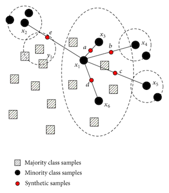
SMOTE is an oversampling method which creates “synthetic” example rather than oversampling by replacements. The minority class is over-sampled by taking each minority class sample and introducing synthetic examples along the line segments joining any/all of the k minority class nearest neighbors. Depending upon the amount of over-sampling required, neighbors from the k nearest neighbors are randomly chosen.
The heart of SMOTE is the construction of the minority classes. The intuition behind the construction algorithm is simple. You have already studied that oversampling causes overfitting, and because of repeated instances, the decision boundary gets tightened. What if you could generate similar samples instead of repeating them? In the original SMOTE paper (linked above) it has been shown that to a machine learning algorithm, these newly constructed instances are not exact copies, and thus it softens the decision boundary and thereby helping the algorithm to approximate the hypothesis more accurately.
However, there are some advantages and disadvantages of SMOTE -
Advantages -
Disadvantages -
There are some variants of SMOTE such as safe-level SMOTE, border-line SMOTE, OSSLDDD-SMOTE, etc. If you want to use SMOTE and its other variants you can check the scikit-learn-contrib module as mentioned before. If you want to learn more about SMOTE, you should check this and this papers.
Let's proceed to the final approach for this tutorial.
There are fields of study dedicated to handling imbalanced datasets. They have their own algorithms, measures, and terminology.
Often creativity and an innovative bent of mind can give you new perspectives to consider when you are dealing with imbalanced data. The following approach can give you a head-start:
Cost-Sensitive Learning: Generally, you use regularization (if you want to learn more about regularization you can check this DataCamp article) for penalizing large coefficients which often appear in Generalized Linear Models (GLM). Although this application varies from model to model. You are considering GLM only for the time being. If you can devise a mechanism which penalizes the classifier each time it does a misclassification. This can help the classifier to learn the hypothesis in a much more detailed manner.
Following are some approaches that you should consider:
So far, you got yourself introduced to the concept of imbalanced data and the kind of problem it creates while designing and developing machine learning models. You also saw several reasons as to why it is crucial to tackle imbalanced data. After that, you studied different approaches that can help you to handle imbalanced datasets effectively. Processing imbalanced data is an active area of research, and it can open new horizons for you to consider new research problems.
A lot of essential concepts in one go! Absolutely amazing!
That is all for this tutorial.
Below are some paper links if you are very keen to study even more about the topic of imbalanced data:
References:
If you want to learn more about data visualization, take DataCamp's "Interactive Data Visualization with Bokeh" taught by Bryan Van de Ven who is one of the developers of Bokeh.
Learn more about Machine Learning
Course
Course
Course
Tutorial
Zoumana Keita
Tutorial
Sayak Paul
Tutorial
Moez Ali
code-along
George Boorman
code-along
Justin Saddlemyer
code-along
Filip Schouwenaars