
Track
Hugging Face Fundamentals
12 hr
Qwen3‑VL‑8B is the most powerful and widely used vision‑language model in the Qwen series, designed for unified understanding of text, images, and video.
It delivers major improvements in text generation, visual reasoning, spatial perception, long‑context handling, and agent interaction, making it suitable for both research and real‑world deployment across edge and cloud environments.
In this tutorial, we will fine‑tune Qwen3‑VL‑8B‑Instruct on electronic schematic diagrams. By training the model to interpret schematic symbols, connections, and spatial relationships, we enable it to accurately understand circuit designs and determine which electronic components need to be added in a real‑world circuit.
You will learn how to:
If Hugging Face is still new to you, the Hugging Face Fundamentals skill track is for you!
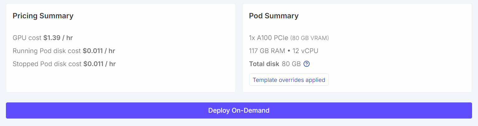
When working with vision–language models, GPU memory becomes a critical constraint. High-resolution images and multimodal encoders can quickly consume VRAM, so using a GPU with ample memory is strongly recommended.
For this tutorial, we will launch a RunPod A100 (80GB) instance using the latest PyTorch image. This setup provides sufficient VRAM headroom for training and avoids unnecessary memory bottlenecks during fine-tuning.
Scroll down to the Pod Template section. Here, select the latest PyTorch image. This is also where you can adjust storage settings and add environment variables.
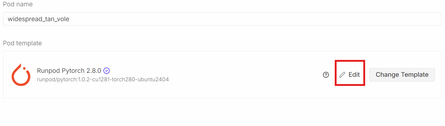
Click Edit, then make the following changes:
HF_TOKEN and set its value to your Hugging Face access token (generate one from the Hugging Face Settings)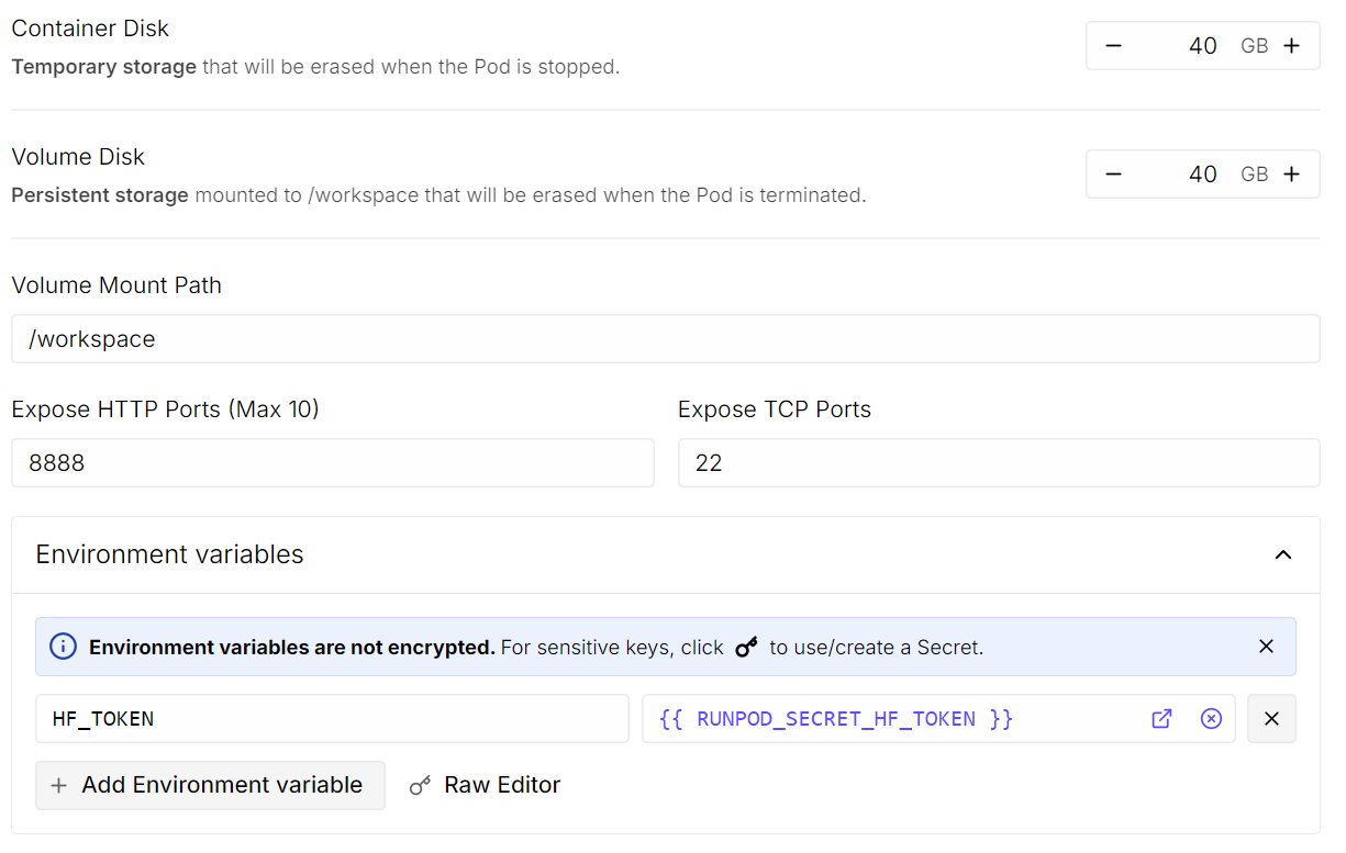
Once done, save the template and deploy the pod.
Once the pod is running:
To install the dependencies, run the following code cell. In Jupyter, an exclamation mark at the beginning tells the notebook to execute the line as a shell command rather than Python code.
!pip -q install -U accelerate datasets pillow sentencepiece safetensors peft
!pip install --quiet "transformers==5.0.0rc1"
!pip install --quiet --no-deps trl
!pip install --no-cache-dir flash-attn --no-build-isolation
Next, set a fixed random seed for reproducibility and enable A100-specific performance optimizations.
import torch
from transformers import set_seed

set_seed(42)

# A100: TF32 gives speedups without changing your bf16 training setup
torch.backends.cuda.matmul.allow_tf32 = True
torch.backends.cudnn.allow_tf32 = True

print("CUDA:", torch.cuda.is_available(), torch.cuda.get_device_name(0) if torch.cuda.is_available() else None)
print("bf16 supported:", torch.cuda.is_available() and torch.cuda.is_bf16_supported())
CUDA: True NVIDIA A100 80GB PCIe
bf16 supported: TrueWe will now load the Open Schematics dataset from the Hugging Face Hub. This dataset contains electronic schematic images along with rich metadata describing each circuit, making it well-suited for vision–language training.
import torch
from datasets import load_dataset

DATASET_ID = "bshada/open-schematics"

ds_all = load_dataset(DATASET_ID, split="train")
print(ds_all)
Dataset({
features: ['schematic', 'image', 'components_used', 'json', 'yaml', 'name', 'description', 'type'],
num_rows: 84470
})The dataset contains 84K+ samples, each pairing a schematic image with structured information, such as component lists and machine-readable formats (JSON and YAML).
Let us inspect a single sample to better understand the dataset structure.
# quick peek
ex = ds_all[0]
print("\nSample keys:", ex.keys())
print("name:", ex.get("name"))
print("type:", ex.get("type"))
print("components_used:", (ex.get("components_used") or [])[:10])
print("has schematic:", bool(ex.get("schematic")))
print("has json/yaml:", bool(ex.get("json")), bool(ex.get("yaml")))
print("image:", ex.get("image"))
Sample keys: dict_keys(['schematic', 'image', 'components_used', 'json', 'yaml', 'name', 'description', 'type'])
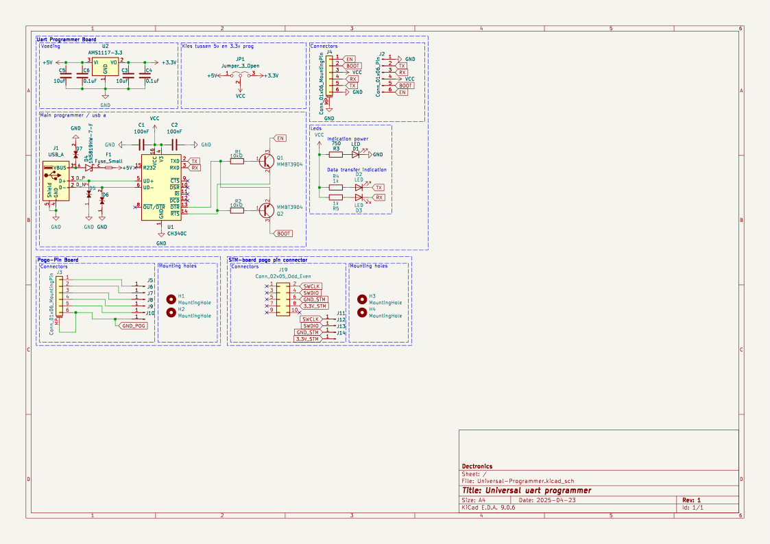
name: TiebeDeclercq/Uart-programmer
type: .kicad_sch
components_used: ['Conn_01x01_Pin', 'Conn_01x06_Pin', 'USB_A', 'Conn_02x05_Odd_Even', 'Conn_01x06_MountingPin', 'C', 'Fuse_Small', 'LED', 'R', 'CH340C']
has schematic: True
has json/yaml: True True
image: <PIL.PngImagePlugin.PngImageFile image mode=RGBA size=1123x794 at 0x7FBC6FD060F0>This confirms that each sample includes a high-resolution schematic image, a component list, and structured representations of the circuit.
We can now render the schematic image directly inside the Jupyter notebook.
ex.get("image")
Finally, we inspect the full list of components used in this schematic.
print(ex.get("components_used"))['Conn_01x01_Pin', 'Conn_01x06_Pin', 'USB_A', 'Conn_02x05_Odd_Even', 'Conn_01x06_MountingPin', 'C', 'Fuse_Small', 'LED', 'R', 'CH340C', 'Jumper_3_Open', 'MountingHole', 'AMS1117-3.3', 'MMBT3904', '1N5819HW-7-F', 'LESD5D5.0CT1G', '+3.3V', '+5V', 'GND', 'VCC']This component list provides clear grounding between the schematic image and the electronic elements present in the circuit.
Before training, we clean and filter the dataset to ensure that each sample contains the minimum information required for vision–language learning. In particular, we focus on retaining examples that have valid component annotations and a corresponding schematic image.
First, we examine how many samples have missing, empty, or invalid components_used entries.
need_cols = [c for c in ["components_used", "schematic", "name", "type"] if c in ds_all.column_names]
ds_small = ds_all.select_columns(need_cols)

missing_key = none_components = empty_components = missing_any = 0
has_schematic_but_missing = 0

for ex in ds_small:
    if "components_used" not in ex:
        missing_key += 1
        missing_any += 1
        if ex.get("schematic"):
            has_schematic_but_missing += 1
        continue

    cu = ex["components_used"]
    bad = (cu is None) or (isinstance(cu, list) and len(cu) == 0)

    if cu is None:
        none_components += 1
    elif isinstance(cu, list) and len(cu) == 0:
        empty_components += 1

    if bad:
        missing_any += 1
        if ex.get("schematic"):
            has_schematic_but_missing += 1

print("\n=== Missing components report ===")
print("Total:", len(ds_all))
print("Missing key:", missing_key)
print("None:", none_components)
print("Empty list:", empty_components)
print("Missing (any):", missing_any)
if "schematic" in need_cols:
    print("Has schematic but missing components:", has_schematic_but_missing)
=== Missing components report ===
Total: 84470
Missing key: 0
None: 47558
Empty list: 8
Missing (any): 47566
Has schematic but missing components: 47566The summary below shows that a large portion of samples contain schematic data but are missing usable component annotations.
To avoid unnecessary memory usage during filtering, we explicitly disable image decoding. This ensures Hugging Face does not load images into memory while applying filters.
from datasets.features import Image as HFImage
ds_all = ds_all.cast_column("image", HFImage(decode=False))
We then define a filter that keeps only samples with a non-empty component list and a valid image reference.
def keep_components_and_image(components_used, image):
    # keep only rows with components
    if not (isinstance(components_used, list) and len(components_used) > 0):
        return False

    # image must exist
    if image is None:
        return False

    # when decode=False, image is dict-like: {"path": ...} or {"bytes": ...}
    if isinstance(image, dict):
        return bool(image.get("path")) or bool(image.get("bytes"))

    return True
Applying this filter significantly reduces the dataset to high-quality, fully usable samples.
ds_clean = ds_all.filter(
    keep_components_and_image,
    input_columns=["components_used", "image"],
)

print("Original:", len(ds_all))
print("Clean:", len(ds_clean))
print("Dropped:", len(ds_all) - len(ds_clean))
Original: 84470
Clean: 33275
Dropped: 51195After filtering, we are left with 33K+ clean samples that contain both valid schematic images and explicit component annotations. This cleaned dataset forms a reliable foundation for the subsequent preprocessing and model training steps.
We now load the Qwen3-VL-8B-Instruct model along with its corresponding processor. This model is a large-scale vision–language model capable of jointly reasoning over images and text, making it well-suited for schematic understanding tasks.
The model is loaded in bfloat16 precision to reduce memory usage while maintaining numerical stability. We also enable Flash Attention 2 for faster and more memory-efficient attention on the A100 GPU. The device_map="auto" option automatically places model layers on the available GPU.
from transformers import Qwen3VLForConditionalGeneration, AutoProcessor

MODEL_ID = "Qwen/Qwen3-VL-8B-Instruct"

model = Qwen3VLForConditionalGeneration.from_pretrained(
    MODEL_ID,
    dtype=torch.bfloat16,
    device_map="auto",
    attn_implementation="flash_attention_2",
)
processor = AutoProcessor.from_pretrained(MODEL_ID)This step defines lightweight utilities for preparing prompts, targets, and images for vision–language training. A single pipeline is used for multiple tasks by switching the TASK variable (components, YAML, JSON, or schematic reconstruction).
Basic safety limits are applied to control target length and image size, helping keep training stable and memory-efficient.
from PIL import Image


TASK = "components"  # "components" | "yaml" | "json" | "schematic"
MAX_TARGET_CHARS = 5000  # safety cap for long targets like schematic/json
MAX_IMAGE_SIDE = 1024          # bigger side
MAX_IMAGE_PIXELS = 1024 * 1024 # safety cap (1.0 MP). raise to 1.5MP if stableThe build_prompt() function constructs the instruction text passed to the model. It uses dataset metadata for context and enforces strict output constraints to reduce hallucination and keep supervision consistent across tasks.
def build_prompt(example):
    # Use dataset fields to give better context (name/type are helpful)
    name = example.get("name") or "Unknown project"
    ftype = example.get("type") or "unknown format"

    if TASK == "components":
        return (
            f"Project: {name}\nFormat: {ftype}\n"
            "From the schematic image, extract all component labels and identifiers exactly as shown "
            "(part numbers, values, footprints, net labels like +5V/GND).\n"
            "Output only a comma-separated list. Do not generalize or add extra text."
        )

    if TASK == "yaml":
        return (
            f"Project: {name}\nFormat: {ftype}\n"
            "From the schematic image, produce YAML metadata for the design.\n"
            "Return valid YAML only. No markdown, no explanations."
        )

    if TASK == "json":
        return (
            f"Project: {name}\nFormat: {ftype}\n"
            "From the schematic image, produce a JSON representation of the schematic structure.\n"
            "Return valid JSON only. No markdown, no explanations."
        )

    if TASK == "schematic":
        return (
            f"Project: {name}\nFormat: {ftype}\n"
            "From the schematic image, reconstruct the raw KiCad schematic content.\n"
            "Return only the schematic text. No markdown, no explanations."
        )

raise ValueError("Unknown TASK")The build_target() function extracts the ground-truth output for the selected task directly from the dataset. The content is returned verbatim to train the model on exact reproduction, not paraphrasing.
def build_target(example):
    if TASK == "components":
        comps = example.get("components_used") or []
        return ", ".join(comps)

    if TASK == "yaml":
        return (example.get("yaml") or "").strip()

    if TASK == "json":
        return (example.get("json") or "").strip()

    if TASK == "schematic":
        return (example.get("schematic") or "").strip()

    raise ValueError("Unknown TASK")
The clamp_text() function applies a hard character limit to targets. This prevents oversized JSON, YAML, or schematic files from causing memory issues during training.
def clamp_text(s: str, max_chars: int = MAX_TARGET_CHARS) -> str:
    s = (s or "").strip()
return s if len(s) <= max_chars else s[:max_chars].rstrip()The _resize_pil() function normalizes and resizes schematic images before processing. It enforces both a maximum side length and a maximum total pixel count, ensuring predictable GPU memory usage while preserving visual detail.
def _resize_pil(pil: Image.Image, max_side: int = MAX_IMAGE_SIDE, max_pixels: int = MAX_IMAGE_PIXELS) -> Image.Image:
    pil = pil.convert("RGB")
    w, h = pil.size

    # Scale down if max side too large
    scale_side = min(1.0, max_side / float(max(w, h)))

    # Scale down if too many pixels (area cap)
    scale_area = (max_pixels / float(w * h)) ** 0.5 if (w * h) > max_pixels else 1.0

    scale = min(scale_side, scale_area)

    if scale < 1.0:
        nw, nh = max(1, int(w * scale)), max(1, int(h * scale))
        pil = pil.resize((nw, nh), resample=Image.BICUBIC)

return pilIn this step, we convert each cleaned dataset sample into a multimodal chat-style format that can be directly consumed by the Qwen vision–language model. This format explicitly aligns the schematic image with a textual instruction and its corresponding target output.
def to_messages(example):
    prompt = build_prompt(example)
    target = clamp_text(build_target(example))

    example["messages"] = [
        {
            "role": "user",
            "content": [
                {"type": "image"},
                {"type": "text", "text": prompt},
            ],
        },
        {
            "role": "assistant",
            "content": [{"type": "text", "text": target}],
        },
    ]
    return example
We shuffle the dataset to remove ordering bias and select a small subset for initial experiments.
The dataset is then mapped through to_messages() to generate multimodal training examples. Finally, image decoding is re-enabled, so that images are loaded only at training time, keeping preprocessing lightweight and memory-efficient.
# Start small (increase later)
train_ds = ds_clean.shuffle(seed=42).select(range(min(800, len(ds_clean)))).map(to_messages)
train_ds = train_ds.cast_column("image", HFImage(decode=True))Before fine-tuning, we evaluate the out-of-the-box performance of the Qwen3-VL 8B Instruct model on our task. This baseline helps us understand how well the pretrained model can extract information from schematic images without any task-specific adaptation.
The run_inference() function performs a single forward pass on one example using the same prompting and image preprocessing logic that will later be used during training.
import torch

def run_inference(model_, example, max_new_tokens=256):
    prompt = build_prompt(example)

    messages = [
        {
            "role": "user",
            "content": [
                {"type": "image", "image": _resize_pil(example["image"])},
                {"type": "text", "text": prompt},
            ],
        }
    ]

    inputs = processor.apply_chat_template(
        messages,
        tokenize=True,
        add_generation_prompt=True,
        return_dict=True,
        return_tensors="pt",
    ).to(model_.device)

    with torch.inference_mode():
        out = model_.generate(**inputs, max_new_tokens=max_new_tokens, do_sample=False)

    gen = out[0][inputs["input_ids"].shape[1]:]
    return processor.decode(gen, skip_special_tokens=True)

baseline_ex = train_ds.shuffle(seed=120).select(range(1))[0]
We first evaluate the model on a randomly selected sample from the training set.
print("\n--- BASELINE OUTPUT ---\n", run_inference(model, baseline_ex))
print("\n--- TARGET (dataset) ---\n", clamp_text(build_target(baseline_ex), 1500))
--- BASELINE OUTPUT ---
J1,Conn_02x11_Odd_Even,CINT6,CINT5,CINT4,CINT3,CINT2,CINT1,CINT0,CINT15,CINT14,CINT13,CINT12,CINT11,CINT10,CINT9,CINT8,CINT7,CINT16,CINT17,CINT18,CINT19,CINT20,CINT21,CINT22,CINT23,CINT24,CINT25,CINT26,CINT27,CINT28,CINT29,CINT30,CINT31,CINT32,CINT33,CINT34,CINT35,CINT36,CINT37,CINT38,CINT39,CINT40,CINT41,CINT42,CINT43,CINT44,CINT45,CINT46,CINT47,CINT48,CINT49,CINT50,CINT51,CINT52,CINT53,CINT54,CINT55,CINT56,CINT57,CINT58,CINT59,CINT60,CINT61,CINT62
--- TARGET (dataset) ---
Conn_02x11_Odd_Even, R_Pack04, GNDIn this example, the model correctly identifies some structural elements but over-generates pin and signal names, while failing to recover the exact component identifiers used in the dataset. I spotted this same pattern throughout more examples when I evaluated them.
Overall, these baseline results show that while the model has strong general visual and textual understanding, it lacks alignment with dataset-specific component annotations. This behavior highlights the need for fine-tuning to reduce hallucinated outputs and improve precision.
This section defines a custom data collator that prepares multimodal chat-style batches for training. It converts each example into model-ready tensors by jointly encoding text and images, while ensuring that loss is computed only on the assistant’s response.
The collator builds two versions of the chat text: a full version (prompt and target) for input encoding, and a prompt-only version to compute prompt token lengths. Using these lengths, all prompt and padding tokens are masked in the labels, so only the assistant output contributes to the loss. Images are resized consistently, and a fixed maximum sequence length is enforced for memory control.
from typing import List, Dict, Any
import torch

MAX_LEN = 1500

def collate_fn(batch: List[Dict[str, Any]]):
    # 1) Build full chat text (includes assistant answer)
    full_texts = [
        processor.apply_chat_template(
            ex["messages"],
            tokenize=False,
            add_generation_prompt=False,
        )
        for ex in batch
    ]

    # 2) Build prompt-only text (up to user turn; generation prompt on)
    prompt_texts = [
        processor.apply_chat_template(
            ex["messages"][:-1],
            tokenize=False,
            add_generation_prompt=True,
        )
        for ex in batch
    ]

    # 3) Images
    images = [_resize_pil(ex["image"]) for ex in batch]

    # 4) Tokenize full inputs ONCE (text + images)
    enc = processor(
        text=full_texts,
        images=images,
        return_tensors="pt",
        padding=True,
        truncation=True,
        max_length=MAX_LEN,
    )

    input_ids = enc["input_ids"]
    pad_id = processor.tokenizer.pad_token_id

    # 5) Compute prompt lengths with TEXT-ONLY tokenization (much cheaper than text+images)
    prompt_ids = processor.tokenizer(
        prompt_texts,
        return_tensors="pt",
        padding=True,
        truncation=True,
        max_length=MAX_LEN,
        add_special_tokens=False,  # chat template already includes special tokens
    )["input_ids"]

    # Count non-pad tokens in prompt
    prompt_lens = (prompt_ids != pad_id).sum(dim=1)

    # 6) Labels: copy + mask prompt tokens + mask padding
    labels = input_ids.clone()
    bs, seqlen = labels.shape

    for i in range(bs):
        pl = int(prompt_lens[i].item())
        pl = min(pl, seqlen)
        labels[i, :pl] = -100

    # Mask padding positions too
    labels[labels == pad_id] = -100

    # If your processor produces pixel_values / image_grid_thw, keep them
    enc["labels"] = labels
    return enc
This collator enables efficient and correct supervision for vision–language fine-tuning.
We will now configure LoRA (Low-Rank Adaptation) to fine-tune the Qwen3-VL model efficiently without updating all model weights. LoRA injects trainable low-rank matrices into selected projection layers, significantly reducing memory usage while preserving performance.
from peft import LoraConfig, TaskType, get_peft_model

lora = LoraConfig(
    r=16,
    lora_alpha=32,
    lora_dropout=0.05,
    bias="none",
    task_type=TaskType.CAUSAL_LM,
    target_modules=[
        "q_proj","k_proj","v_proj","o_proj",
        "gate_proj","up_proj","down_proj"
    ],
)
We then define the training configuration using SFTConfig, setting batch size, learning rate, precision, and logging options suitable for stable fine-tuning on the A100 GPU.
from trl import SFTTrainer, SFTConfig

args = SFTConfig(
    output_dir=f"qwen3vl-open-schematics-{TASK}-lora",
    num_train_epochs=1,
    per_device_train_batch_size=2,
    gradient_accumulation_steps=4,
    gradient_checkpointing=False,
    learning_rate=1e-4,
    warmup_steps=10,
    weight_decay=0.01,
    max_grad_norm=1.0,
    bf16=True,
    fp16=False,
    lr_scheduler_type="cosine",
    logging_steps=10,
    report_to="none",
    remove_unused_columns=False,
)
Finally, we initialize the SFTTrainer, combining the model, dataset, custom collator, and LoRA configuration to begin supervised fine-tuning.
trainer = SFTTrainer(
    model=model,
    args=args,
    train_dataset=train_ds,
    data_collator=collate_fn,
    peft_config=lora
)We now start the fine-tuning process using the configured trainer.
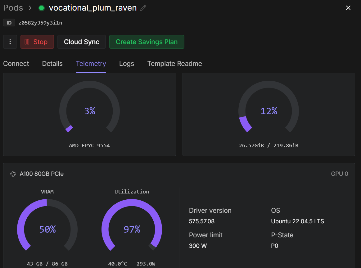
trainer.train()Once training begins, you can monitor the RunPod telemetry dashboard. On an A100 80GB instance, the process typically uses around 40–45 GB of VRAM and reaches near-full GPU utilization, indicating efficient hardware usage.
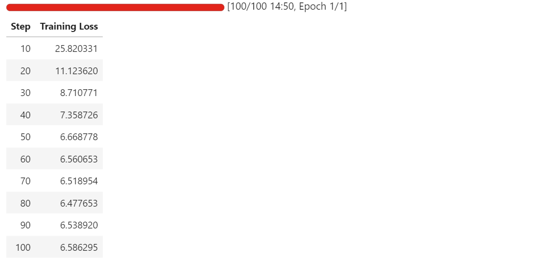
As training progresses, you should observe the training loss decreasing steadily before stabilizing. In our case, the loss converges and plateaus at approximately 6.5, which serves as a baseline indicator that the model has adapted to the schematic component extraction task.
At this point, the LoRA adapters are successfully fine-tuned and ready for evaluation and export.
After fine-tuning completes, we first save the trained LoRA adapters and the associated processor locally.
out_dir = trainer.args.output_dir # from your SFTConfig/TrainingArguments
trainer.save_model(out_dir) # saves model/adapters into output_dir
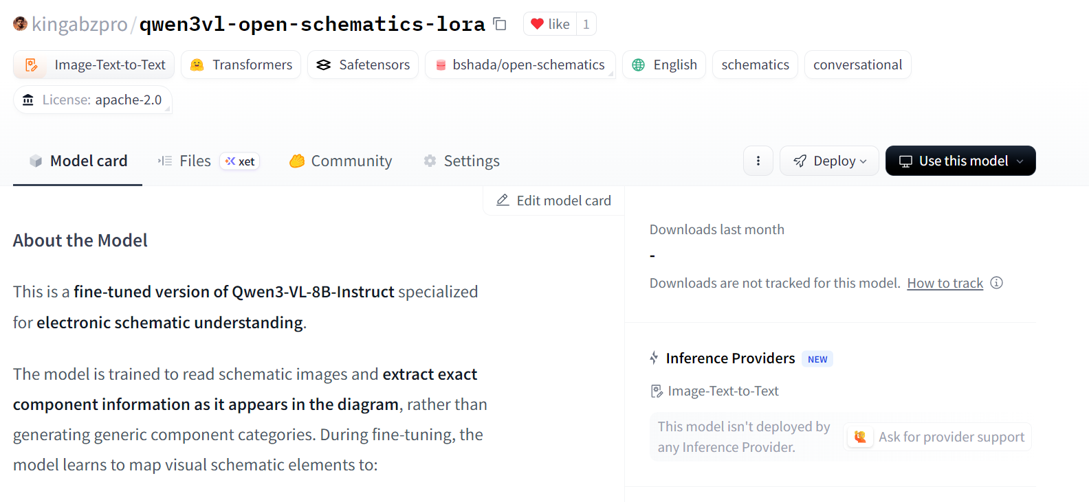
processor.save_pretrained(out_dir) # save processor (tokenizer + image processor)Next, we publish the fine-tuned model to the Hugging Face Hub. This allows the adapters and processor to be reused for inference or further fine-tuning.
import os

repo_id = "kingabzpro/qwen3vl-open-schematics-lora" # replace with your username/repo

# Push model/adapters
trainer.model.push_to_hub(
    repo_id,
    token=os.getenv("HF_TOKEN"),
)

# Push processor
processor.push_to_hub(
    repo_id,
    token=os.getenv("HF_TOKEN"),
)
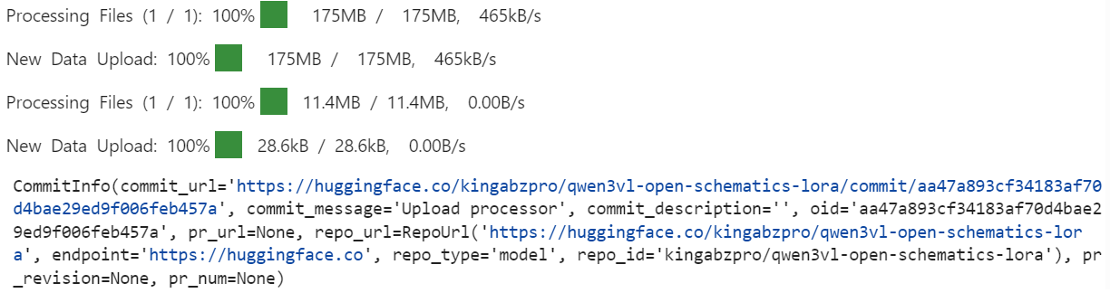
Once the upload is complete, the fine-tuned LoRA adapters and processor are available publicly in the specified repository.
After fine-tuning, we reload the model and processor directly from the Hugging Face Hub. This ensures that evaluation is performed using the exported LoRA adapters, exactly as they would be used in a real inference setting.
model = Qwen3VLForConditionalGeneration.from_pretrained(
    repo_id,
    dtype=torch.bfloat16,
    device_map="auto",
    attn_implementation="flash_attention_2",
)
processor = AutoProcessor.from_pretrained(repo_id)
```
We now repeat the same inference procedure used during the baseline evaluation, allowing for a direct comparison between pre-fine-tuning and post-fine-tuning behavior.
```python
baseline_ex = train_ds.shuffle(seed=120).select(range(1))[0]
print("\n--- FINETUNED OUTPUT ---\n", run_inference(model, baseline_ex))
print("\n--- TARGET (dataset) ---\n", clamp_text(build_target(baseline_ex), 1500))
--- FINETUNED OUTPUT ---
Conn_02x11_0dd_Even, P3.3V
--- TARGET (dataset) ---
Conn_02x11_Odd_Even, R_Pack04, GNDCompared to the baseline, the fine-tuned model produces a much shorter and more focused output, avoiding the large-scale over-generation of pin names and inferred signals.
While the prediction is still incomplete and contains minor errors, it shows clear movement toward dataset-aligned component identifiers.
We will now evaluate a second example to confirm this behavior.
baseline_ex = train_ds.shuffle(seed=170).select(range(1))[0]
print("\n--- FINETUNED OUTPUT ---\n", run_inference(model, baseline_ex))
print("\n--- TARGET (dataset) ---\n", clamp_text(build_target(baseline_ex), 1500))
--- FINETUNED OUTPUT ---
ATMEGA328P-PU, +5V, GND, R, C, C16MHz, SERVO_A, SERVO_B, SERVO_C, SERVO_D, SERVO_E, SERVO_F, SERVO_G
--- TARGET (dataset) ---
+5V, 7.62MM-3P, 7.62MM-3P_1, 7.62MM-3P_2, 7.62MM-3P_3, 7.62MM-3P_4, 7.62MM-3P_5, 7.62MM-3P_6, ATMEGA328P-PU, ATMEGA328P-PU_1, GND, MBB02070C1002FCT00, MBB02070C1002FCT00_1, Unknown_0_-806, X49SD16MSD2SC, Y5P102K2KV16CC0224, Y5P102K2KV16CC0224_1, Y5P102K2KV16CC0224_2Here, the fine-tuned model correctly identifies core components such as the microcontroller and power nets, and significantly reduces irrelevant signal-level hallucinations. However, it still abstracts or generalizes some components instead of reproducing the exact dataset-specific identifiers.
Overall, these results demonstrate that fine-tuning successfully suppresses over-generation and improves alignment with schematic-level component extraction. While precision can be further improved with additional epochs, larger training sets, or stricter output constraints, the post-fine-tuning behavior represents a clear and measurable improvement over the baseline.
If you encounter any issues running the code in this tutorial, please refer to the accompanying notebook.
Vision–language models are fundamentally different from text-only models, and treating them the same almost always leads to poor results.
If you are not careful, it is very easy to run into out-of-memory errors even with a batch size of one, or to fine-tune a model that appears to train but fails to actually learn the task. This is something I learned the hard way.
What ultimately made the difference was paying attention to the details that matter specifically for multimodal training.
Resizing images to safe bounds, cleaning the dataset to remove broken or unusable samples, and ensuring that only valid image–text pairs are passed to the model are all essential steps. Skipping any of these quickly leads to instability or wasted compute.
On the modeling side, using only the relevant LoRA target layers helped keep training efficient and focused, while careful tuning of training arguments improved convergence without increasing memory pressure.
Optimizing for the A100 GPU, enabling Flash Attention, and using bfloat16 allowed training to remain stable while significantly reducing runtime. In practice, these optimizations cut training time nearly in half without sacrificing quality.
The final results show that even a strong pretrained vision–language model benefits greatly from domain-specific fine-tuning. With the right preprocessing, configuration, and hardware-aware optimizations, it is possible to adapt large multimodal models reliably and efficiently.
If you’re interested in further practicing fine-tuning, I recommend taking the Fine-Tuning with Llama 3 course.
LLM Courses
Track
Course
Course
Tutorial
Abid Ali Awan
Tutorial
Abid Ali Awan
Tutorial
Bex Tuychiev
Tutorial
Abid Ali Awan
Tutorial
Abid Ali Awan
Tutorial
Abid Ali Awan