Fine-Tuning Ministral 3: A Step-by-Step Guide to Training a Vision-Language Model for X-Ray Classification

Ministral 3 is a new family of edge-optimized multimodal models available in 3B, 8B, and 14B sizes, each offering Base, Instruct, and Reasoning variants with full vision support. 

Designed to deliver strong frontier-level performance while remaining lightweight enough for local and private deployment, Ministral 3 bridges advanced capabilities with practical hardware constraints, its flagship 14B Instruct model fits in 24GB VRAM in FP8 and rivals larger systems like Mistral Small 3.2 24B. With a large 256k context window, robust multilingual coverage, native function calling, strong system-prompt adherence, and Apache 2.0 open licensing. 

In this tutorial, we will fine-tune the Ministral 3 14B Instruct model on a bone-fracture X-ray dataset to improve its ability to detect fractures and classify their categories accurately. 

You will learn how to:

1. Load the dataset from Kaggle.
2. Convert it into a Hugging Face dataset.
3. Create a clear training prompt for X-ray classification.
4. Set up the Ministral 3 14B vision-language training pipeline.
5. Fine-tune the model and save the checkpoint.
6. Load the trained model adopter for inference.
7. Compare results before and after fine-tuning.

If you’re eager to learn more about the Mistral AI models, I recommend our guide Mistral 3 and Mistral 3 Large tutorial. 

Disclaimer: This tutorial demonstrates a technical fine-tuning process for educational purposes only. The resulting model is not intended for medical or clinical use and should not be relied upon for diagnosis, decision-making, or patient care.

1. Environment Setup for Ministral 3 Vision-Language Fine-Tuning

Even though we are fine-tuning the 14B model, vision language training requires significantly more memory than text-only fine-tuning. The image encoder increases GPU load, which means we need access to an A100 GPU with 80 GB of VRAM to run this process smoothly. 

For this project, I am using Runpod and launching an A100 pod.

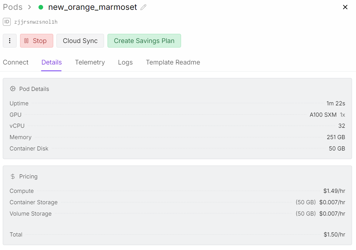
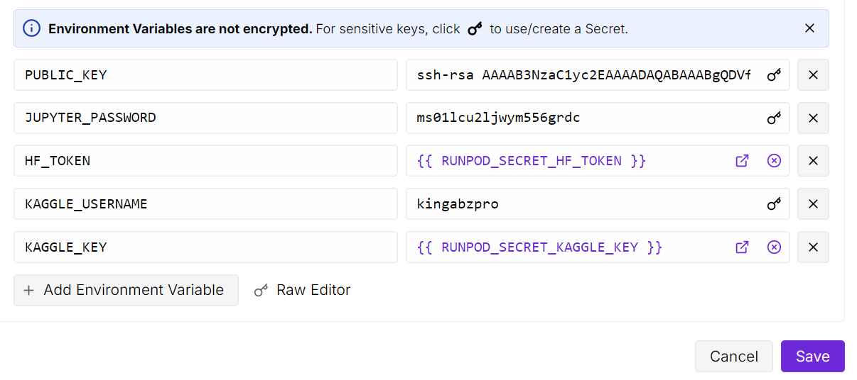
After launching the pod, increase the container storage to 50 GB. Then add the environment variables for both Kaggle and Hugging Face API keys. 

Kaggle will allow us to download the bone X-ray dataset directly, and Hugging Face will allow us to push our fine-tuned LoRA adapter back to the model hub.

Next, open the JupyterLab instance and create a fresh notebook. Before training, we need to install all required Python packages. 

Make sure the Transformers library is updated to the latest version, because Ministral 3 support was added recently, and older builds will not load the model correctly.

! pip install --upgrade --quiet bitsandbytes datasets evaluate hf_transfer peft scikit-learn matplotlib Pillow kaggle ipywidgets
!pip install --quiet git+https://github.com/huggingface/transformers.git@bf3f0ae70d0e902efab4b8517fce88f6697636ce
!pip install --quiet --no-deps trl==0.22.2

Once everything is installed, you are ready to load the dataset, prepare the collator, and begin fine-tuning.

2. Downloading the Bone Fracture Dataset from Kaggle

In the next step, we set up a root folder for our dataset and use the Kaggle Python API to download the Bone Break Classification Image dataset. 

This dataset contains various bone fracture categories in X-ray format and will be used to fine-tune Ministral 3 for visual classification.

import os
import glob
from kaggle.api.kaggle_api_extended import KaggleApi

DATA_ROOT = "/bone-break"
os.makedirs(DATA_ROOT, exist_ok=True)

kaggle_dataset = "pkdarabi/bone-break-classification-image-dataset"

# Initialize and authenticate Kaggle API (it will read KAGGLE_USERNAME / KAGGLE_KEY)
api = KaggleApi()
api.authenticate()

# Download and unzip the dataset using the Python API
api.dataset_download_files(
    kaggle_dataset,
    path=DATA_ROOT,
    unzip=True,
)

You can view the dataset on Kaggle here:

Dataset URL: https://www.kaggle.com/datasets/pkdarabi/bone-break-classification-image-dataset

3. Building a Hugging Face Dataset

The downloaded dataset is not organized in the usual structure. Each fracture category contains both a training folder and a testing folder inside it. 

So first, we need a method to loop through every class folder, separate the two splits, and then create a combined Hugging Face dataset with a clean train and test mapping.

import glob, os
from typing import Any, Dict, List

from datasets import Dataset, DatasetDict, Features, ClassLabel, Image

inner_root = os.path.join(
    DATA_ROOT, "Bone Break Classification", "Bone Break Classification"
)

classes = []
train_records: List[Dict[str, Any]] = []
test_records: List[Dict[str, Any]] = []

for class_name in sorted(os.listdir(inner_root)):
    class_dir = os.path.join(inner_root, class_name)
    if not os.path.isdir(class_dir):
        continue

    classes.append(class_name)

    for split_name, split_key in [("Train", "train"), ("Test", "test")]:
        split_dir = os.path.join(class_dir, split_name)
        if not os.path.isdir(split_dir):
            continue

        for ext in ("*.png", "*.jpg", "*.jpeg"):
            for img_path in glob.glob(os.path.join(split_dir, ext)):
                rec = {"image": img_path, "label_name": class_name}
                if split_key == "train":
                    train_records.append(rec)
                else:
                    test_records.append(rec)

print("Classes:", classes)
print("Train samples:", len(train_records))
print("Test samples:", len(test_records))

We have a total of 10 classifications, with 989 training samples and 140 testing samples.

Classes: ['Avulsion fracture', 'Comminuted fracture', 'Fracture Dislocation', 'Greenstick fracture', 'Hairline Fracture', 'Impacted fracture', 'Longitudinal fracture', 'Oblique fracture', 'Pathological fracture', 'Spiral Fracture']
Train samples: 989
Test samples: 140

We will now encode the labels for the Hugging Face dataset so that each label class will be considered as class labels and each image will be treated as image features. 

We will create two datasets: one for training and one for testing. Finally, we will combine them into a single dataset that contains both training and testing subsets.

# Encode labels
classes = sorted(list(set(classes)))
label2id = {name: i for i, name in enumerate(classes)}

for rec in train_records:
    rec["label"] = label2id[rec["label_name"]]
for rec in test_records:
    rec["label"] = label2id[rec["label_name"]]

features = Features(
    {
        "image": Image(),
        "label": ClassLabel(names=classes),
    }
)

train_ds = Dataset.from_list(
    [{"image": r["image"], "label": r["label"]} for r in train_records],
    features=features,
)
test_ds = Dataset.from_list(
    [{"image": r["image"], "label": r["label"]} for r in test_records],
    features=features,
)

data = DatasetDict({"train": train_ds, "test": test_ds})
data

Here is the overview of the dataset. 

DatasetDict({
    train: Dataset({
        features: ['image', 'label'],
        num_rows: 989
    })
    test: Dataset({
        features: ['image', 'label'],
        num_rows: 140
    })
})

4. Exploring Class Distribution and Sample X-Ray Images

Before fine-tuning, it is helpful to understand how balanced the dataset is and what the images look like. We will begin by checking how many training samples exist for each fracture category.

from collections import Counter

label_names = data["train"].features["label"].names
label_ids = data["train"]["label"]

counts = Counter(label_ids)
print("Training Class counts:")
for lbl_id, cnt in counts.items():
    print(f"{lbl_id:2d} ({label_names[lbl_id]}): {cnt}")

FRACTURE_CLASSES = label_names

The categories are fairly balanced, although the overall sample size is small for a complex vision classification task. 

For now, we will proceed with this dataset, but results should be interpreted with realistic expectations due to the limited sample volume.

Training Class counts:
 0 (Avulsion fracture): 109
 1 (Comminuted fracture): 134
 2 (Fracture Dislocation): 137
 3 (Greenstick fracture): 106
 4 (Hairline Fracture): 101
 5 (Impacted fracture): 75
 6 (Longitudinal fracture): 68
 7 (Oblique fracture): 69
 8 (Pathological fracture): 116
 9 (Spiral Fracture): 74

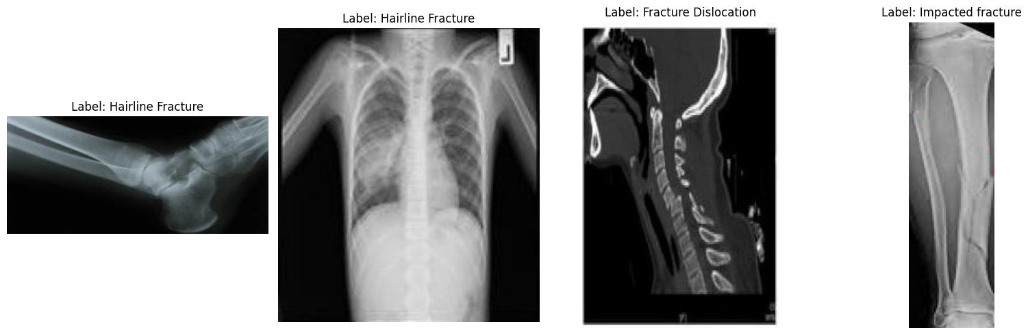
Next, let us view a few random images to better understand the dataset visually.

import matplotlib.pyplot as plt
from datasets import Image

# Cast the 'image' column to Hugging Face Image feature
dataset_images = data.cast_column("image", Image())

# Select random samples from the training set
samples = dataset_images["train"].shuffle(seed=420).select(range(4))

# Plot
fig, axes = plt.subplots(1, 4, figsize=(16, 5))

for i, sample in enumerate(samples):
    img_object = sample["image"]              # PIL Image
    label_id = sample["label"]               # int
    label_name = label_names[label_id]       # string

    axes[i].imshow(img_object)
    axes[i].set_title(f"Label: {label_name}")
    axes[i].axis("off")

plt.tight_layout()
plt.show()

Looking at the sample images, we can see differences in size, resolution, orientation, and scan quality. This does not affect fine-tuning a vision language model, but it can influence how consistently the model learns each fracture category. 

Detecting a fracture visually is often straightforward, but classifying it into one of ten subtle medical fracture types requires more structured data than what is provided here.

5. Prompt Design for Bone Fracture Classification

Next, we need to decide how we want the model to behave. For this task, our goal is very strict: given an X-ray image, the model should output only one fracture class name and nothing else. No explanations, no markdown, no extra text.

We will write a clear instruction prompt and then use it to build a messages column in the dataset. 

PROMPT = f"""
You are a radiology assistant specialised in bone fracture classification.

You must classify the X-ray image into exactly ONE of the following classes:
{", ".join(FRACTURE_CLASSES)}

Rules:
- Reply with ONLY the class name.
- No explanations, no extra words, no markdown, no punctuation.
- Output must be EXACTLY one of: {", ".join(FRACTURE_CLASSES)}
""".strip()


from typing import Dict, Any

def convert_to_conversation(example: Dict[str, Any]) -> Dict[str, Any]:
    conversation = [
        {
            "role": "user",
            "content": [
                {"type": "text",  "text": PROMPT},
                {"type": "image"},     # no image bytes here
            ],
        },
        {
            "role": "assistant",
            "content": [
                {"type": "text", "text": FRACTURE_CLASSES[example["label"]]},
            ],
        },
    ]
    example["messages"] = conversation
    return example




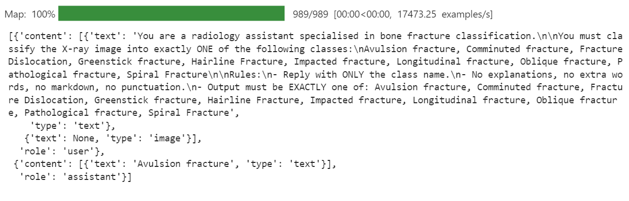
formatted_data = data["train"].map(convert_to_conversation)
formatted_data["messages"][0]

This creates a messages column where each record now contains a complete mini conversation: the instruction plus the correct fracture class. This is exactly what the vision language model will see during fine tuning.

6. Loading the Ministral 3 Vision-Language Model

Now we load the BF16 version of the Ministral-3 14B Instruct model from the Hugging Face Hub, along with processor. The processor bundles together the tokenizer and the image pre-processing pipeline, which is required for vision language inputs.

import torch
from transformers import AutoProcessor, AutoModelForImageTextToText, BitsAndBytesConfig

model_id = "mistralai/Ministral-3-14B-Instruct-2512-BF16"


model_kwargs = dict(
    attn_implementation="eager",
    torch_dtype=torch.bfloat16,
    device_map="auto",
)

model = AutoModelForImageTextToText.from_pretrained(model_id, **model_kwargs)
processor = AutoProcessor.from_pretrained(model_id)

# Use right padding to avoid issues during training
processor.tokenizer.padding_side = "right"

7. Setting Up Custom Chat Template

The original chat template provided by Mistral AI is designed for long, conversational use cases. For this project, that became a problem. The model started to focus on the long role instructions and system text, and it ignored the actual goal, which is predicting a single bone fracture class from the X-ray.

To fix this, we define a shorter vision language template that only keeps the important parts: the user instruction and the assistant's answer. This reduces noise and helps the model learn a clean mapping from image to class label.

SHORT_VLM_TEMPLATE = r"""{{ bos_token }}[INST]
{% for message in messages if message['role'] == 'user' -%}
  {%- for content in message['content'] -%}
    {%- if content['type'] == 'text' -%}
{{ content['text'] }}

    {%- elif content['type'] == 'image' -%}
[IMG]
    {%- endif -%}
  {%- endfor -%}
{%- endfor -%}
[/INST]{% if not add_generation_prompt %}
  {%- for message in messages if message['role'] == 'assistant' -%}
{{ message['content'][0]['text'] }}{{ eos_token }}
  {%- endfor -%}
{%- endif %}"""


# Attach to processor / tokenizer
processor.chat_template = SHORT_VLM_TEMPLATE
processor.tokenizer.chat_template = SHORT_VLM_TEMPLATE

8. Testing Ministral 3 (Pre-Fine-Tuning)

Before we start fine-tuning, it is useful to test the original Ministral 3 14B Instruct model to create a baseline. 

First, we give the model a random image from the dataset and ask a general question, just to see how it understands the content of the X-ray.

image = formatted_data[200]["image"]

messages = [
    {"role": "user", "content": [
        {"type": "text", "text": "What is the image about?"},
        {"type": "image"},
        
    ]}
]

input_text = processor.apply_chat_template(messages, add_generation_prompt = True)
inputs = processor(
    image,
    input_text,
    add_special_tokens = False,
    return_tensors = "pt",
).to(device="cuda", dtype=torch.bfloat16)

from transformers import TextStreamer
text_streamer = TextStreamer(processor, skip_prompt = True)
_ = model.generate(**inputs, streamer = text_streamer, max_new_tokens = 1000,
                   use_cache = True, temperature = 1.5, min_p = 0.1)

As a result, the model understood the general content of the X ray, but then drifted into descriptions that were not reliable for medical use.

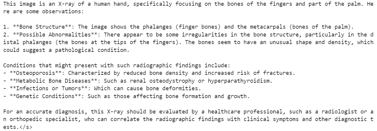
Next, we try something closer to our final objective. We give the same image, but this time we use our strict fracture classification prompt instead of an open question.

image = formatted_data[200]["image"]

messages = [
    {"role": "user", "content": [
        {"type": "text", "text": PROMPT},
        {"type": "image"},
        
    ]}
]

input_text = processor.apply_chat_template(messages, add_generation_prompt = True)
inputs = processor(
    image,
    input_text,
    add_special_tokens = False,
    return_tensors = "pt",
).to(device="cuda", dtype=torch.bfloat16)

from transformers import TextStreamer
text_streamer = TextStreamer(processor, skip_prompt = True)
_ = model.generate(**inputs, streamer = text_streamer, max_new_tokens = 1000,
                   use_cache = True, temperature = 1.5, min_p = 0.1

For this sample, the model responded with:

Hairline Fracture</s>

Now we check the actual ground truth label for the same image.

FRACTURE_CLASSES[formatted_data[200]["label"]]

This returns:

'Comminuted fracture'

So, the model followed the instruction format correctly and produced a single class name, but the classification itself was wrong. 

This is exactly why we need fine-tuning. The base model has strong vision understanding, but it has not been trained specifically to distinguish between detailed bone fracture types. 

In the next steps, we will fine-tune it on our fracture dataset to improve that behaviour.

9. Configuring LoRA for Efficient Ministral 3 Fine-Tuning

Next, we set up LoRA to fine-tune the Ministral 3 model efficiently without updating all parameters. This configuration targets the main attention and MLP projection layers used in a Mistral-style vision-language model.

from peft import LoraConfig, TaskType, get_peft_model

# LoRA config for a Mistral-style VLM used as a causal LM
peft_config = LoraConfig(
    task_type=TaskType.CAUSAL_LM,
    r=16,
    lora_alpha=32,
    lora_dropout=0.05,
    bias="none",
    target_modules=[
        "q_proj",
        "k_proj",
        "v_proj",
        "o_proj",
        "gate_proj",
        "up_proj",
        "down_proj",
    ],
    modules_to_save=None,
)

Next, we define the supervised fine-tuning (SFT) training arguments.

This configuration controls the full training process, including how batches are handled, memory optimization, learning rate behavior, logging, saving strategy, and integration with Hugging Face Hub. 

from trl import SFTConfig

args = SFTConfig(
    output_dir="ministral-3-bone-fracture",            
    num_train_epochs=1,                       
    per_device_train_batch_size=2,                           
    per_device_eval_batch_size=2,                            
    gradient_accumulation_steps=4,                           
    gradient_checkpointing=True,                             
    optim="adamw_8bit",                               
    logging_steps=0.1,                                        
    save_strategy="epoch",                                                                                                             
    learning_rate=2e-4,                             
    bf16=True,
    fp16=False,
    max_grad_norm=0.3,                                       
    warmup_steps=25,                                       
    lr_scheduler_type="linear",                              
    push_to_hub=True,                                        
    report_to="none",
    gradient_checkpointing_kwargs={"use_reentrant": False},  
    dataset_kwargs={"skip_prepare_dataset": True},           
    remove_unused_columns = False,                           
    label_names=["labels"],                                  
)

10. Building a Vision-Language Data Collator for Training

For fine-tuning a vision-language model like Ministral 3, we need a custom data collator that can batch images and chat-style text together in a consistent format. 

The collator below takes care of: setting up the tokenizer and pad token, applying the chat template, tokenizing text and images jointly, enforcing a safe maximum sequence length, and creating labels where padding and image tokens are masked out (-100) so they don’t affect the loss. 

from typing import Any, Dict, List
import torch

# --- One-time processor setup ---
tokenizer = processor.tokenizer
tokenizer.padding_side = "right"

# Ensure we have a pad token
if tokenizer.pad_token is None:
    tokenizer.add_special_tokens({"pad_token": tokenizer.eos_token})

pad_token_id = tokenizer.pad_token_id
image_token_id = getattr(processor, "image_token_id", None)

# Hard cap for sequence length
MAX_SEQ_LEN = 2048 


def collate_fn(examples: List[Dict[str, Any]]) -> Dict[str, torch.Tensor]:
    """
    Collate function for VLM fine-tuning.

    Each example must contain:
      - "image": a PIL image
      - "messages": chat-style conversation (list[dict])
    """
    images = [ex["image"] for ex in examples]
    conversations = [ex["messages"] for ex in examples]

    # Build chat prompts for the whole batch
    chat_texts = processor.apply_chat_template(
        conversations,
        add_generation_prompt=False,
        tokenize=False,
    )

    # Tokenize + process images
    batch = processor(
        text=chat_texts,
        images=images,
        padding="longest", 
        truncation=True,
        max_length=MAX_SEQ_LEN,
        return_tensors="pt",
    )

    # Labels: same as input_ids but mask pad & image tokens
    labels = batch["input_ids"].clone()

    if pad_token_id is not None:
        labels[labels == pad_token_id] = -100

    if image_token_id is not None and image_token_id != pad_token_id:
        labels[labels == image_token_id] = -100

    batch["labels"] = labels
    return batch

11. Fine-Tuning Ministral 3 Using TRL

With the LoRA adapter, training config, and data collator ready, we can now plug everything into trl’s SFTTrainer. 

This trainer handles the full supervised fine-tuning loop for our vision-language Ministral 3 model, using our formatted dataset, LoRA config, and custom collate function for image–text batches.

from trl import SFTTrainer

trainer = SFTTrainer(
    model=model,
    args=args,
    train_dataset=formatted_data,
    peft_config=peft_config,
    processing_class=processor,
    data_collator=collate_fn,
)

Run the code below to start the training process. 

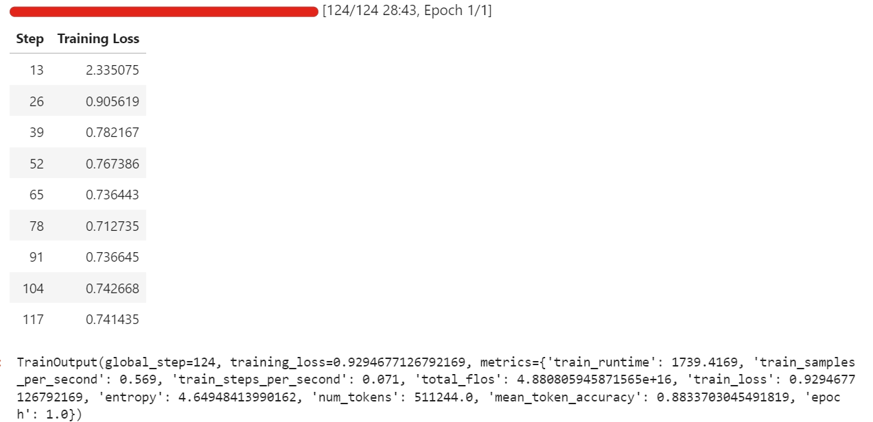
trainer.train()

During my run, fine-tuning used around 57 GB of VRAM, and a bit more during evaluation steps that run every few iterations. In practice, this means you can fine-tune this setup comfortably on hardware with under 70 GB of VRAM.

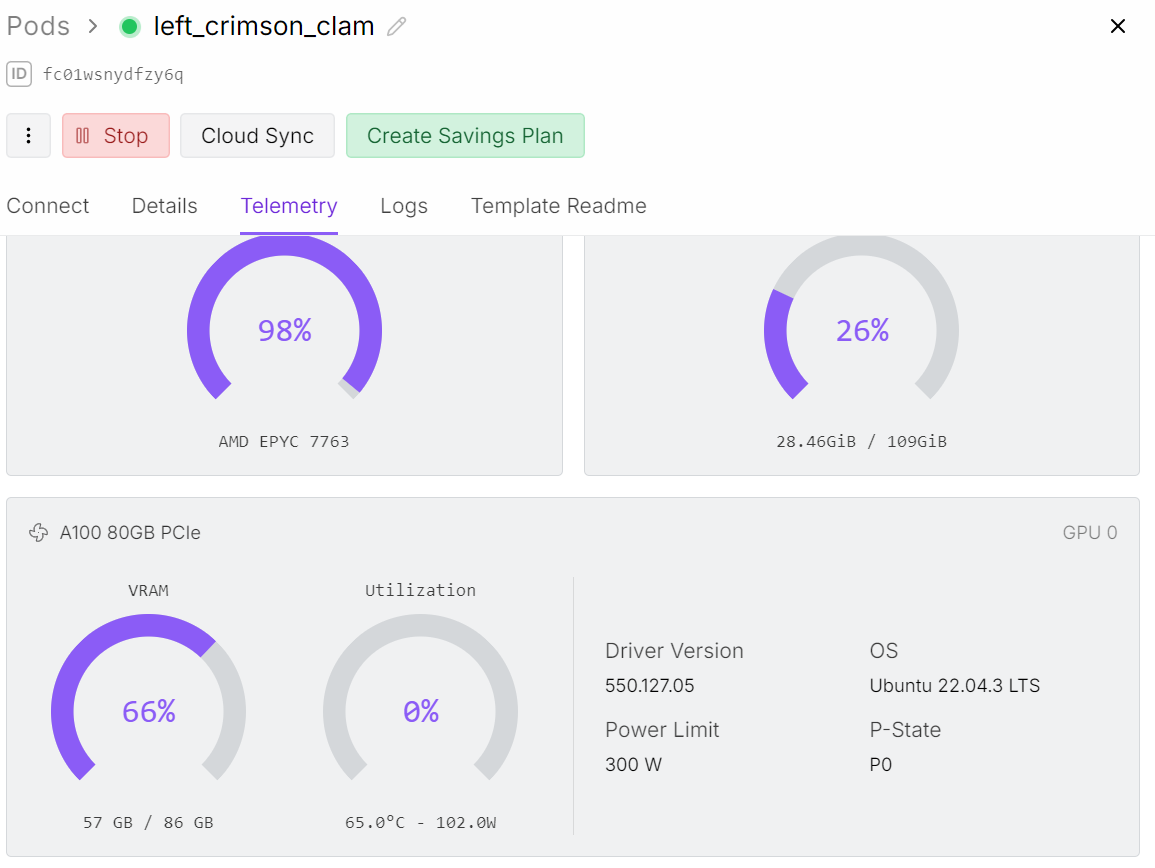
The full training took around half an hour, and the training loss decreased steadily over time, which is a good sign that the model is learning from the dataset.

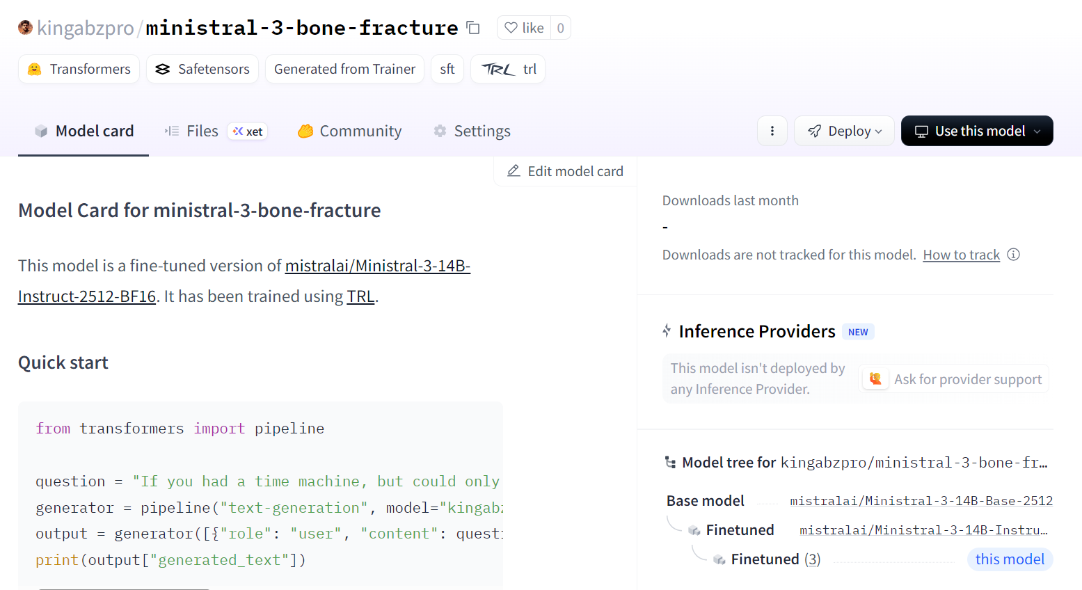
Once training is complete, we save the adapted model to the Hugging Face Hub. This will create a new repository and push all required files so that you can reload and run the fine-tuned model from any environment.

trainer.save_model()

You can view the model at kingabzpro/ministral-3-bone-fracture. 

12. Evaluating the Fine-Tuned Ministral 3 Model

Now we load the fine-tuned model and processor from the Hugging Face Hub. Under the hood, this will download the saved LoRA adapter, load the base Ministral 3 checkpoint, and merge the adapter into the base model so it is ready for inference.

import torch
from transformers import AutoProcessor, AutoModelForImageTextToText, BitsAndBytesConfig

model_id = "kingabzpro/ministral-3-bone-fracture"


model_kwargs = dict(
    attn_implementation="eager",
    dtype=torch.bfloat16,
    device_map="auto",
)

model = AutoModelForImageTextToText.from_pretrained(model_id, **model_kwargs)
processor = AutoProcessor.from_pretrained(model_id)

processor.tokenizer.padding_side = "left"

To keep the comparison fair, we first reuse the same image that we tested before fine tuning (index 200) and run it through the inference pipeline with our strict classification prompt.

image = formatted_data[200]["image"]

messages = [
    {"role": "user", "content": [
        {"type": "text", "text": PROMPT},
        {"type": "image"},
        
    ]}
]

input_text = processor.apply_chat_template(messages, add_generation_prompt = True)
inputs = processor(
    image,
    input_text,
    add_special_tokens = False,
    return_tensors = "pt",
).to(device="cuda", dtype=torch.bfloat16)

from transformers import TextStreamer
text_streamer = TextStreamer(processor, skip_prompt = True)
_ = model.generate(**inputs, streamer = text_streamer, max_new_tokens = 100)

We achieved a perfect result. No extra post-processing was needed. The model followed the prompt rules and produced the correct class directly.

Comminuted fracture</s>

Next, we try another random sample from the dataset to confirm that this behaviour is not limited to one example.

image = formatted_data[400]["image"]

messages = [
    {"role": "user", "content": [
        {"type": "text", "text": PROMPT},
        {"type": "image"},
        
    ]}
]

input_text = processor.apply_chat_template(messages, add_generation_prompt = True)
inputs = processor(
    image,
    input_text,
    add_special_tokens = False,
    return_tensors = "pt",
).to(device="cuda", dtype=torch.bfloat16)

from transformers import TextStreamer
text_streamer = TextStreamer(processor, skip_prompt = True)
_ = model.generate(**inputs, streamer = text_streamer, max_new_tokens = 100)

Model output:

Greenstick fracture</s>

Ground truth:

FRACTURE_CLASSES[formatted_data[400]["label"]]

Output:

'Greenstick fracture'

Again, the prediction is correct and fully aligned with the label.

With these checks, we can say that our Ministral 3 14B model has been successfully fine-tuned on the bone fracture X-ray dataset and is now able to follow the instruction prompt and produce accurate single-class predictions for these examples.

Final Thoughts

Fine-tuning the Ministral 3 model requires patience and steady adjustments. It genuinely took me two full days to understand why the model was not training the way I expected and why, despite being a relatively small model, it was still pushing my GPU into out-of-memory errors. 

The main reason was simple, but easy to overlook. This is not just a language model. It is a vision language model, which means it carries an image encoder that adds extra memory usage. 

Larger image resolutions lead directly to higher VRAM consumption. Reducing image size or starting with smaller batches makes the training process far more stable.

Another issue I ran into was using the default chat template. It was far too long and structured for this type of task. The model was spending more effort fitting the template formatting instead of learning how to read the images and produce a clear fracture classification. 

Once I simplified the prompt into a direct instruction format, the model finally began to respond to the visual input correctly instead of shaping every answer like a full chat response.

I also assumed that because the model has strong vision abilities, it would naturally perform well on medical scans. That assumption slowed me down. Calling it “MedGemma” in my head was not fair to the model or the process. It is not a specialised medical model out of the box, and expecting it to behave like one without proper training was my mistake.

In the end, I worked past each hurdle and turned what I learned into this guide. The goal is to help you avoid the same confusion and get to meaningful results faster. 

“With smaller images, simpler prompts, and realistic expectations, Ministral 3 can be fine-tuned for X-ray understanding in a much smoother and more reliable way.”

If you’re keen to get more hands-on practice with fine-tuning, I recommend the Fine-Tuning with Llama 3 course.