When you’re picking up Excel for the first time, you’ll probably encounter a few functions that are key in referencing and searching for data. In most cases, this will be using the Lookup functions in Excel.

In this article, we’ll cover the various functions related to looking up information in Excel and explain how you can use them through examples. If you’re looking to sharpen your Excel skills across all areas, be sure to check out our Excel Fundamentals skill track.

What are Excel Lookup Functions?

Lookup functions in Excel allow users to search for specific data within a dataset and return corresponding information from another column or row. They are essential in data analysis for referencing, cross-referencing, and extracting meaningful insights from large or complex datasets.

Why are Lookup Functions Important? 

Lookup functions are great for efficient data retrieval. Efficient data retrieval is crucial for productivity, especially when dealing with large spreadsheets or automating reporting workflows. Lookup functions reduce manual searching, ensure consistency, and enable scalable data solutions.

For example, imagine you have a sales table with thousands of rows and columns, and you need to find the total sales for a specific product or region. 

Without lookup functions, you’d need to manually search through each row to find the relevant information, which is time-consuming and prone to human error.

Learn more about these functions in our Data Preparation in Excel course.

Types of Lookup Functions in Excel

Excel offers multiple lookup functions, each with unique strengths tailored for different use cases. Understanding the differences between these functions can significantly improve your ability to manage and analyze data efficiently.

Let’s look at some common types of functions below.

1. LOOKUP

Source: Microsoft

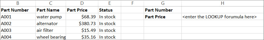
The original lookup function is the most basic and works with sorted arrays. It searches for a value in a single row or column and returns a value from the same position in another row or column. It only supports approximate matches.

2. VLOOKUP (Vertical Lookup)

Source: Microsoft

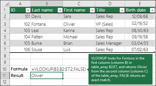
VLOOKUP is one of the most widely used functions in legacy Excel workbooks. It searches for a value in the first column of a table and returns a value in the same row from a specified column. 

It supports both exact and approximate matching but has limitations, such as an inability to search to the left and performance issues with large datasets.

3. HLOOKUP (Horizontal Lookup)

Source: HLOOKUP Tutorial

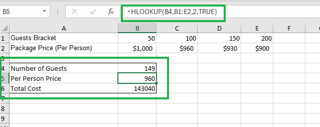
HLOOKUP works similarly to VLOOKUP but searches for a value in the first row of a table and returns a value from a specified row. It's useful when your data is organized horizontally rather than vertically.

You should consider using HLOOKUP over VLOOKUP when your data is organized in rows instead of columns.

4. INDEX and MATCH

The INDEX and MATCH method features the use of a powerful combination of two functions:

• INDEX returns the value of a cell based on row and column numbers.
• MATCH returns the position of a value in a row or column. Used together, they offer more flexibility than VLOOKUP and are preferred in complex scenarios because they support left-to-right and right-to-left lookups and don’t require sorted data.

5. XLOOKUP

Introduced in Excel 2019 and Microsoft 365, XLOOKUP is the modern replacement for VLOOKUP and HLOOKUP. It allows for exact or approximate matching, works horizontally or vertically, and supports error handling, making it the most versatile lookup function to date.

The LOOKUP Function

Let’s start by exploring the LOOKUP function in excel, exploring the syntax and parameters, the vector form, and a worked example. 

Syntax and parameters

=LOOKUP(lookup_value, lookup_vector, [result_vector])

Here are some explanations:

• lookup_value: The value to search for.
• lookup_vector: The single row or column to search.
• result_vector (optional): The range containing the value to return.

Using the vector form

The vector form is commonly used and requires both fields lookup_vector and result_vector to be the same size.

Explanation with examples

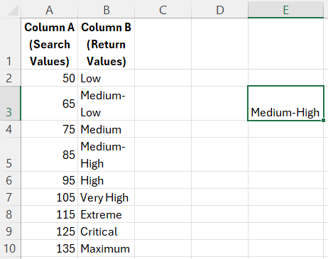
=LOOKUP(90, A2:A10, B2:B10)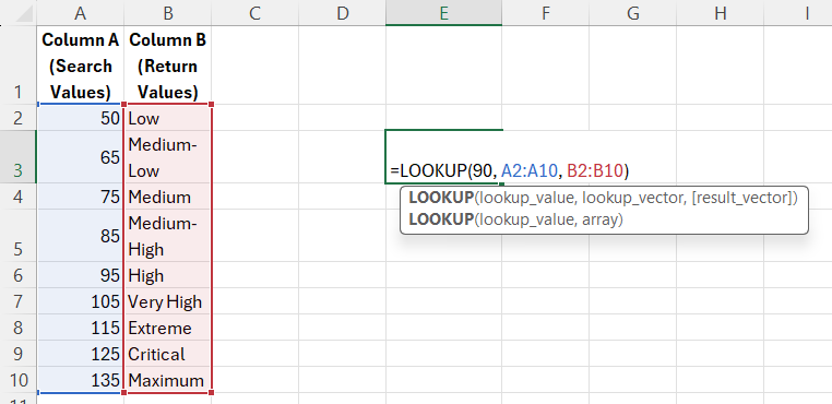

This function searches for the largest value less than or equal to 90 in A2:A10, then returns the corresponding value from B2:B10.

In this case, only row 5 would match the parameters we have set. Therefore, the output of the function would produce the “Medium-High” result.

Limitations of the LOOKUP function

• Requirement for sorted data: The lookup_vector must be sorted in ascending order.
• Approximate match behavior: Does not support exact matches—returns the closest value less than or equal to lookup_value.

The VLOOKUP Function

Nex is the VLOOKUP function, which is one of the most commonly used functions in legacy versions of Excel. 

Syntax and parameters

VLOOKUP(lookup_value, table_array, col_index_num, [range_lookup])

• lookup_value: The value to search for in the first column of the table_array.
• table_array: The table range to search.
• col_index_num: The column number to return a value from.
• range_lookup: Optional; TRUE for approximate match, FALSE for exact.

How to use VLOOKUP: Step-by-step guide with examples

Now, let’s quickly go through how this function works using an example.

We’ll use the following function in a simple dataset.

=VLOOKUP("John", A2:C10, 3, FALSE)

This function will look for any entries that belong to John and output his salary amount.

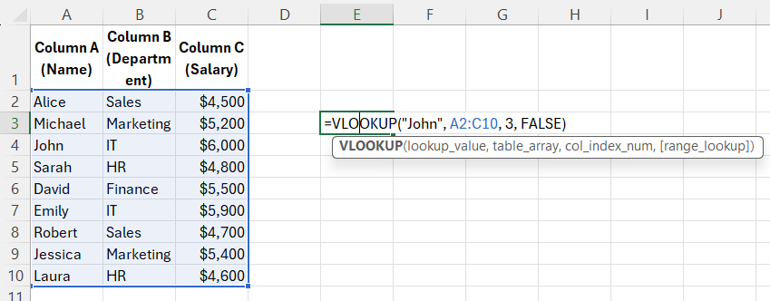
Searches for "John" in column A and returns the value from the third column (column C) in the same row.

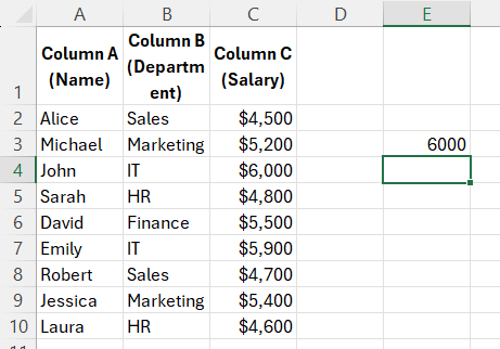
As expected, the VLOOKUP function output is 6000, which matches row 6, which is the value we were looking for, since it belongs to John.

Exact vs approximate matches

Exact matches are the most commonly used type of match in VLOOKUP. This means that the function will only return a result if it finds an exact match for the lookup value in the first column of the specified range.

For example, if we were to use an exact match when searching for John's salary, the VLOOKUP function would only return a result if there was a row with "John" in the first column and his salary in the second column.

On the other hand, approximate matches allow for some flexibility in finding values. This is useful when working with numerical data or data that may have small variations (for example, due to rounding or formatting).

To summarize:

• Exact (FALSE): Finds a precise match.
• Approximate (TRUE): Requires sorted data and finds the nearest match.

Common errors and troubleshooting

When working with VLOOKUP for the first time, some common errors may arise. 

Handling #N/A errors

One of the most common errors when using VLOOKUP is #N/A, which stands for "Not Available." This usually occurs when the value being searched for cannot be found in the specified range.

This can also be caused by a missing lookup_value or unsorted data when using an approximate match.

To troubleshoot this error, double-check that your search value is spelled correctly and exists in the first column of the range you are searching in. Also, make sure that your data is sorted in ascending order if using an approximate match.

Another potential issue is a mismatch between data types. For example, if one column contains numbers represented as text and another column contains actual numbers, VLOOKUP may not work properly.

Column index number issues

Another error that may occur is the #REF! Error. If col_index_num exceeds the number of columns in table_array, a #REF! error occurs.

The HLOOKUP Function

To search for a value in the top row of a table and return a value from a specified row in the same column, the HLOOKUP function is often the best choice. Let’s see how it works.

Syntax and parameters

HLOOKUP(lookup_value, table_array, row_index_num, [range_lookup])

• lookup_value: The value to search for in the first row.
• table_array: The table to search.
• row_index_num: The row number to return a value from.
• range_lookup: TRUE (approximate) or FALSE (exact).

How to use HLOOKUP: Step-by-step guide with examples

=HLOOKUP("Q1", A1:D3, 2, FALSE)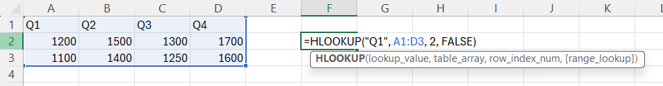

The HLOOKUP function above searches for "Q1" in row 1 and returns the value from row 2 in the same column. 

Let’s run the function and see the results.

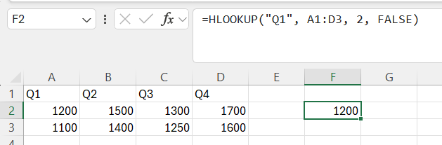
As you can see above, the function should return 1200. Since the function looks for the value found in row 2 based on the value specified in row 1, 1200 is the right output we are looking for.

The INDEX and MATCH Functions

Next, let’s see how the INDEX and MATCH functions in Excel combine to look up values. 

Syntax and example usage

=INDEX(array, row_num, [column_num])

The INDEX function returns the value at a specific row and column in a given range.

=MATCH(lookup_value, lookup_array, [match_type])

The MATCH function returns the relative position of lookup_value in lookup_array.

Using INDEX and MATCH together

When both the INDEX and MATCH functions are used together, they provide a powerful tool for looking up values in a table or range. This combination allows you to specify the exact location of the value you want to return, rather than having to manually input the row and column numbers.

Let’s look at an example:

=INDEX(B2:B10, MATCH("John", A2:A10, 0))

This combination finds the row where "John" appears in A2:A10, then returns the corresponding value from B2:B10.

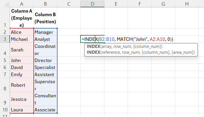
Let’s see what the function will output.

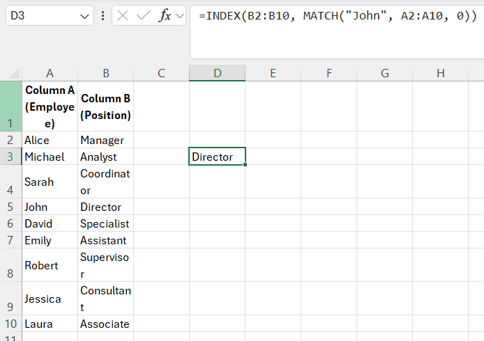
When the two functions are used together, they achieve the same result as using the VLOOKUP function. However, using INDEX and MATCH allows for more flexibility in choosing which column to return from, as well as being able to search in multiple columns.

The XLOOKUP Function (Excel 2019 and Later)

Finally, let’s look at one of the newest Excel lookup functions, XLOOKUP.

Syntax and parameters

XLOOKUP(lookup_value, lookup_array, return_array, [if_not_found], [match_mode], [search_mode])

Practical examples

We’ll be applying the function on a simple dataset and example.

=XLOOKUP("John", A2:A10, B2:B10, "Not Found")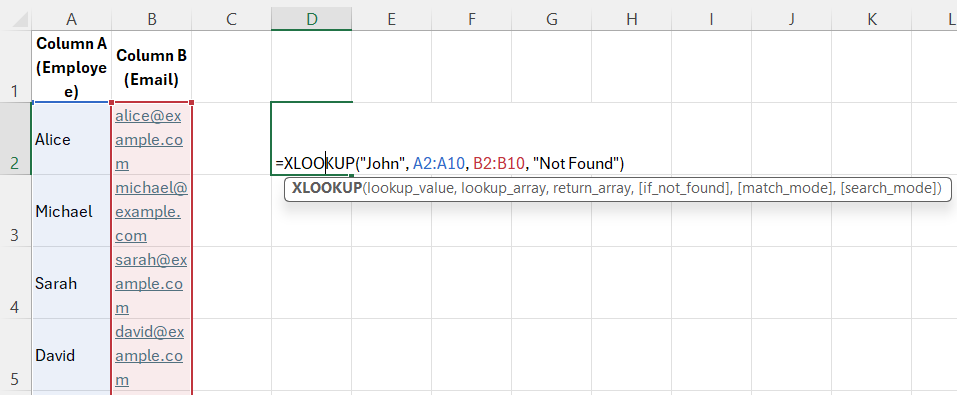

The function above searches for "John" in A2:A10 and returns the value from B2:B10; returns "Not Found" if missing.

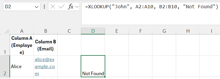
Looking at the output from the formula given above, we can see that the “Not Found” output was shown. This means that there is not such entry with the employee name of “John”.

Comparison: LOOKUP vs. VLOOKUP vs. XLOOKUP

Let’s put all these functions together to see how they match up and look at their differences.

Conclusion

Lookup functions are essential tools in Excel for efficient data retrieval. While LOOKUP, VLOOKUP, and HLOOKUP have their uses, INDEX/MATCH and XLOOKUP provide more flexibility and power. Understanding when and how to use each can significantly enhance your spreadsheet efficiency and analytical capabilities.

If you’re looking for more resources on Excel, our Data Preparation in Excel course would be a great place to start. To master the foundations of Excel, our Excel Fundamentals skill track is the best place to start. You can also check out our Excel tutorials on Basic Excel Formulas or Vlookup from other sheets in Excel as well.