Market Basket Analysis using R

You are a data scientist (or becoming one!), and you get a client who runs a retail store. Your client gives you data for all transactions that consists of items bought in the store by several customers over a period of time and asks you to use that data to help boost their business. Your client will use your findings to not only change/update/add items in inventory but also use them to change the layout of the physical store or rather an online store. To find results that will help your client, you will use Market Basket Analysis (MBA) which uses Association Rule Mining on the given transaction data.

In this tutorial you will learn:

• What is Association Rule Mining and Applications
• What is the APRIORI Algorithm?
• How to implement MBA/Association Rule Mining using R with Visualizations

Association Rule Mining

Association Rule Mining is used when you want to find an association between different objects in a set, find frequent patterns in a transaction database, relational databases or any other information repository. The applications of Association Rule Mining are found in Marketing, Basket Data Analysis (or Market Basket Analysis) in retailing, clustering and classification. It can tell you what items do customers frequently buy together by generating a set of rules called Association Rules. In simple words, it gives you output as rules in form if this then that. Clients can use those rules for numerous marketing strategies:

• Changing the store layout according to trends
• Customer behavior analysis
• Catalogue design
• Cross marketing on online stores
• What are the trending items customers buy
• Customized emails with add-on sales

Consider the following example:

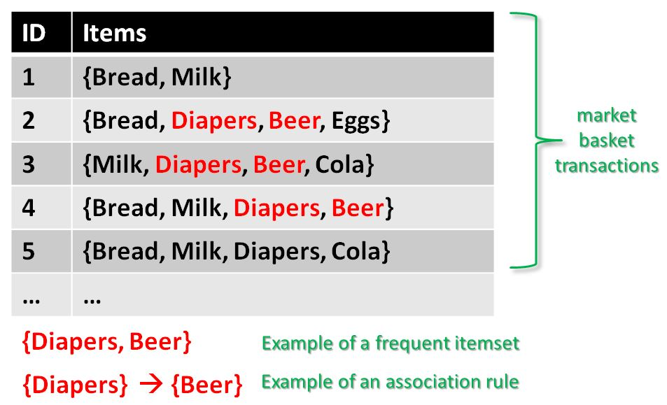
Given is a set of transaction data. You can see transactions numbered 1 to 5. Each transaction shows items bought in that transaction. You can see that Diaper is bought with Beer in three transactions. Similarly, Bread is bought with milk in three transactions making them both frequent item sets. Association rules are given in the form as below:

$A=>B[Support,Confidence]$

The part before $=>$ is referred to as if (Antecedent) and the part after $=>$ is referred to as then (Consequent).

Where A and B are sets of items in the transaction data. A and B are disjoint sets.

$Computer=>Anti-virus Software[Support=20\%,confidence=60\%]$

Above rule says:

1. 20% transaction show Anti-virus software is bought with purchase of a Computer
2. 60% of customers who purchase Anti-virus software is bought with purchase of a Computer

In the following section you will learn about the basic concepts of Association Rule Mining:

Basic Concepts of Association Rule Mining

1. Itemset: Collection of one or more items. K-item-set means a set of k items.

2. Support Count: Frequency of occurrence of an item-set

3. Support (s): Fraction of transactions that contain the item-set 'X'

   $Support(X)=\frac{frequency(X)}{N}$

For a Rule A=>B, Support is given by:

$Support(A=>B)=\frac{frequency(A,B)}{N}$

Note: P(AUB) is the probability of A and B occurring together. P denotes probability.

Go ahead, try finding the support for Milk=>Diaper as an exercise.

1. Confidence (c): For a rule A=>B Confidence shows the percentage in which B is bought with A.

$Confidence(A=>B)=\frac{P(A\cap B)}{P(A)}=\frac{frequency(A,B)}{frequency(A)}$

The number of transactions with both A and B divided by the total number of transactions having A.

$Confidence(Bread=>Milk)=\frac{3}{4}=0.75=75\%$

Now find the confidence for Milk=>Diaper.

Note: Support and Confidence measure how interesting the rule is. It is set by the minimum support and minimum confidence thresholds. These thresholds set by client help to compare the rule strength according to your own or client's will. The closer to threshold the more the rule is of use to the client.

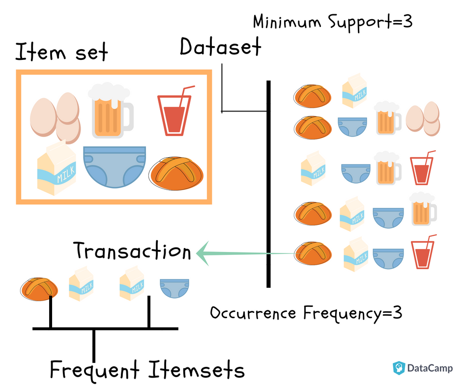
1. Frequent Itemsets: Item-sets whose support is greater or equal than minimum support threshold (min_sup). In above example min_sup=3. This is set on user choice.

2. Strong rules: If a rule A=>B[Support, Confidence] satisfies min_sup and min_confidence then it is a strong rule.

3. Lift: Lift gives the correlation between A and B in the rule A=>B. Correlation shows how one item-set A effects the item-set B.

$Lift(A=>B)=\frac{Support}{Supp(A)Supp(B)}$

For example, the rule {Bread}=>{Milk}, lift is calculated as:

$support(Bread)=\frac{4}{5}=0.8$

$support(Milk)=\frac{4}{5}=0.8$

$Lift(Bread=>Milk)=\frac{0.6}{0.8*0.8}=0.9$

• If the rule had a lift of 1,then A and B are independent and no rule can be derived from them.

• If the lift is > 1, then A and B are dependent on each other, and the degree of which is given by ift value.

• If the lift is < 1, then presence of A will have negative effect on B.

Goal of Association Rule Mining

When you apply Association Rule Mining on a given set of transactions T your goal will be to find all rules with:

1. Support greater than or equal to min_support
2. Confidence greater than or equal to min_confidence

APRIORI Algorithm

In this part of the tutorial, you will learn about the algorithm that will be running behind R libraries for Market Basket Analysis. This will help you understand your clients more and perform analysis with more attention. If you already know about the APRIORI algorithm and how it works, you can get to the coding part.

Association Rule Mining is viewed as a two-step approach:

1. Frequent Itemset Generation: Find all frequent item-sets with support >= pre-determined min_support count

2. Rule Generation: List all Association Rules from frequent item-sets. Calculate Support and Confidence for all rules. Prune rules that fail min_support and min_confidence thresholds.

Frequent Itemset Generation is the most computationally expensive step because it requires a full database scan.

Among the above steps, Frequent Item-set generation is the most costly in terms of computation.

Above you have seen the example of only 5 transactions, but in real-world transaction data for retail can exceed up to GB s and TBs of data for which an optimized algorithm is needed to prune out Item-sets that will not help in later steps. For this APRIORI Algorithm is used. It states:

Any subset of a frequent itemset must also be frequent. In other words, No superset of an infrequent itemset must be generated or tested

It is represented in Itemset Lattice which is a graphical representation of the APRIORI algorithm principle. It consists of k-item-set node and relation of subsets of that k-item-set.

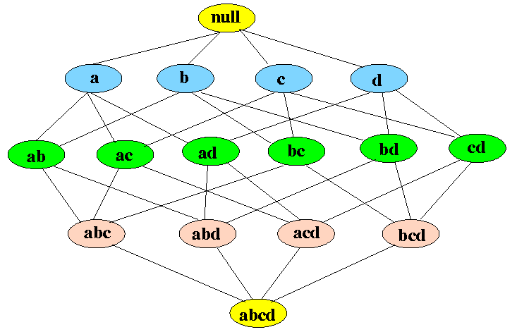
You can see in above figure that in the bottom is all the items in the transaction data and then you start moving upwards creating subsets till the null set. For d number of items size of the lattice will become $2^d$. This shows how difficult it will be to generate Frequent Item-set by finding support for each combination. The following figure shows how much APRIORI helps to reduce the number of sets to be generated:

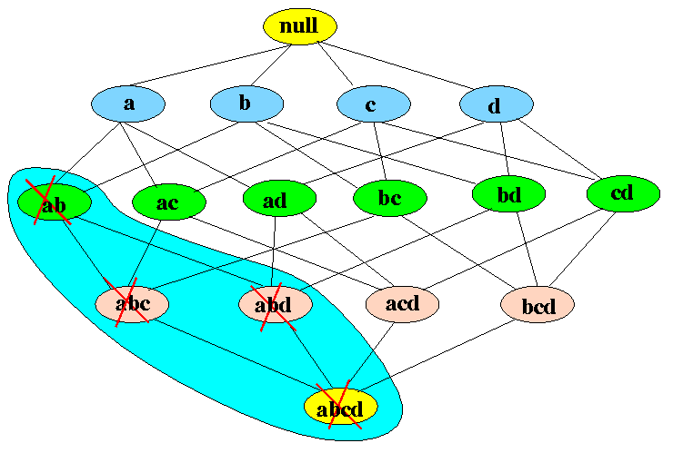
If item-set {a,b} is infrequent then we do not need to take into account all its super-sets.

Let's understand this by an example. In the following example, you will see why APRIORI is an effective algorithm and also generate strong association rules step by step. Follow along on with your notebook and pen!

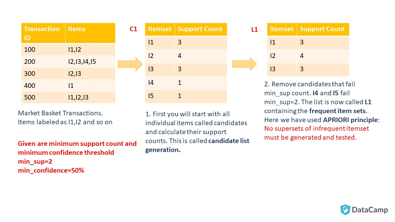
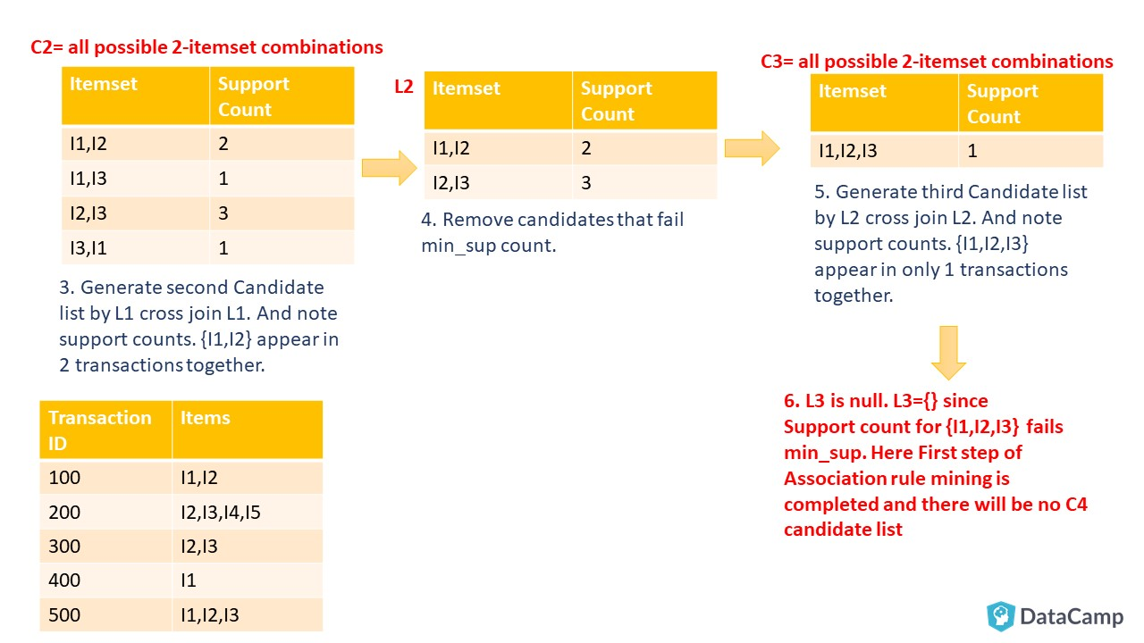
As you can see, you start by creating Candidate List for the 1-itemset that will include all the items, which are present in the transaction data, individually. Considering retail transaction data from real-world, you can see how expensive this candidate generation is. Here APRIORI plays its role and helps reduce the number of the Candidate list, and useful rules are generated at the end. In the following steps, you will see how we reach the end of Frequent Itemset generation, that is the first step of Association rule mining.

Your next step will be to list all frequent itemsets. You will take the last non-empty Frequent Itemset, which in this example is L2={I1, I2},{I2, I3}. Then make all non-empty subsets of the item-sets present in that Frequent Item-set List. Follow along as shown in below illustration:

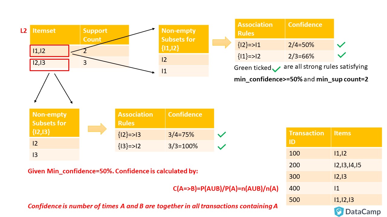
You can see above there are four strong rules. For example, take ${I2}=>I3$ having confidence equal to 75% tells that 75% of people who bought I2 also bought I3.

You have now learned a complete APRIORI algorithm which is one of the most used algorithms in data mining. Let's get on to the code, phewww!

Implementing MBA/Association Rule Mining using R

In this tutorial, you will use a dataset from the UCI Machine Learning Repository. The dataset is called Online-Retail, and you can download it from here. The dataset contains transaction data from 01/12/2010 to 09/12/2011 for a UK-based registered non-store online retail. The reason for using this and not R dataset is that you are more likely to receive retail data in this form on which you will have to apply data pre-processing.

Dataset Description

• Number of Rows:541909
• Number of Attributes:08

Attribute Information

• InvoiceNo: Invoice number. Nominal, a 6-digit integral number uniquely assigned to each transaction. If this code starts with letter 'c', it indicates a cancellation. +StockCode: Product (item) code. Nominal, a 5-digit integral number uniquely assigned to each distinct product.
• Description: Product (item) name. Nominal.
• Quantity: The quantities of each product (item) per transaction. Numeric.
• InvoiceDate: Invoice Date and time. Numeric, the day and time when each transaction was generated. Example from dataset: 12/1/2010 8:26
• UnitPrice: Unit price. Numeric, Product price per unit in sterling.
• CustomerID: Customer number. Nominal, a 5-digit integral number uniquely assigned to each customer.
• Country: Country name. Nominal, the name of the country where each customer resides.

Loading Libraries

First, you will load the libraries required. A short description of the libraries (taken from Here) is given in the following table, so you know what each library does:

#install and load package arules
#install.packages("arules")
library(arules)
#install and load arulesViz
#install.packages("arulesViz")
library(arulesViz)
#install and load tidyverse
#install.packages("tidyverse")
library(tidyverse)
#install and load readxml
#install.packages("readxml")
library(readxl)
#install and load knitr
#install.packages("knitr")
library(knitr)
#load ggplot2 as it comes in tidyverse
library(ggplot2)
#install and load lubridate
#install.packages("lubridate")
library(lubridate)
#install and load plyr
#install.packages("plyr")
library(plyr)
library(dplyr)

Data Pre-processing

Use read_excel(path to file) to read the dataset from the downloaded file into R. Give your complete path to file including filename in read_excel(path-to-file-with-filename)

#read excel into R dataframe
retail <- read_excel('D:/Documents/Online_Retail.xlsx')
#complete.cases(data) will return a logical vector indicating which rows have no missing values. Then use the vector to get only rows that are complete using retail[,].
retail <- retail[complete.cases(retail), ]
#mutate function is from dplyr package. It is used to edit or add new columns to dataframe. Here Description column is being converted to factor column. as.factor converts column to factor column. %>% is an operator with which you may pipe values to another function or expression
retail %>% mutate(Description = as.factor(Description))

retail %>% mutate(Country = as.factor(Country))

#Converts character data to date. Store InvoiceDate as date in new variable
retail$Date <- as.Date(retail$InvoiceDate)
#Extract time from InvoiceDate and store in another variable
TransTime<- format(retail$InvoiceDate,"%H:%M:%S")
#Convert and edit InvoiceNo into numeric
InvoiceNo <- as.numeric(as.character(retail$InvoiceNo))

NAs introduced by coercion

#Bind new columns TransTime and InvoiceNo into dataframe retail
cbind(retail,TransTime)

cbind(retail,InvoiceNo)

#get a glimpse of your data
glimpse(retail)

Observations: 406,829
Variables: 9
$ InvoiceNo   <chr> "536365", "536365", "536365", "536365", "536365", "536365", "53...
$ StockCode   <chr> "85123A", "71053", "84406B", "84029G", "84029E", "22752", "2173...
$ Description <chr> "WHITE HANGING HEART T-LIGHT HOLDER", "WHITE METAL LANTERN", "C...
$ Quantity    <dbl> 6, 6, 8, 6, 6, 2, 6, 6, 6, 32, 6, 6, 8, 6, 6, 3, 2, 3, 3, 4, 4,...
$ InvoiceDate <dttm> 2010-12-01 08:26:00, 2010-12-01 08:26:00, 2010-12-01 08:26:00,...
$ UnitPrice   <dbl> 2.55, 3.39, 2.75, 3.39, 3.39, 7.65, 4.25, 1.85, 1.85, 1.69, 2.1...
$ CustomerID  <dbl> 17850, 17850, 17850, 17850, 17850, 17850, 17850, 17850, 17850, ...
$ Country     <chr> "United Kingdom", "United Kingdom", "United Kingdom", "United K...
$ Date        <date> 2010-12-01, 2010-12-01, 2010-12-01, 2010-12-01, 2010-12-01, 20...

Now, dataframe retail will contain 10 attributes, with two additional attributes Date and Time.

Before applying MBA/Association Rule mining, we need to convert dataframe into transaction data so that all items that are bought together in one invoice are in one row. You can see in glimpse output that each transaction is in atomic form, that is all products belonging to one invoice are atomic as in relational databases. This format is also called as the singles format.

What you need to do is group data in the retail dataframe either by CustomerID, CustomerID, and Date or you can also group data using InvoiceNo and Date. We need this grouping and apply a function on it and store the output in another dataframe. This can be done by ddply.

The following lines of code will combine all products from one InvoiceNo and date and combine all products from that InvoiceNo and date as one row, with each item, separated by ,

library(plyr)
#ddply(dataframe, variables_to_be_used_to_split_data_frame, function_to_be_applied)
transactionData <- ddply(retail,c("InvoiceNo","Date"),
                       function(df1)paste(df1$Description,
                       collapse = ","))
#The R function paste() concatenates vectors to character and separated results using collapse=[any optional charcater string ]. Here ',' is used

transactionData

Next, as InvoiceNo and Date will not be of any use in the rule mining, you can set them to NULL.

#set column InvoiceNo of dataframe transactionData  
transactionData$InvoiceNo <- NULL
#set column Date of dataframe transactionData
transactionData$Date <- NULL
#Rename column to items
colnames(transactionData) <- c("items")
#Show Dataframe transactionData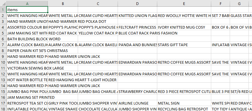
transactionData

This format for transaction data is called the basket format. Next, you have to store this transaction data into a .csv (Comma Separated Values) file. For this, write.csv()

write.csv(transactionData,"D:/Documents/market_basket_transactions.csv", quote = FALSE, row.names = FALSE)
#transactionData: Data to be written
#"D:/Documents/market_basket.csv": location of file with file name to be written to
#quote: If TRUE it will surround character or factor column with double quotes. If FALSE nothing will be quoted
#row.names: either a logical value indicating whether the row names of x are to be written along with x, or a character vector of row names to be written.

See if your transaction data has the correct form:

Next, you have to load this transaction data into an object of the transaction class. This is done by using the R function read.transactions of the arules package.

The following line of code will take transaction data file D:/Documents/market_basket_transactions.csv which is in basket format and convert it into an object of the transaction class.

tr <- read.transactions('D:/Documents/market_basket_transactions.csv', format = 'basket', sep=',')
#sep tell how items are separated. In this case you have separated using ','

When you run the above lines of code you may get lots of EOF within quoted string in your output, don't worry about it.

If you already have transaction data in a dataframe, use the following line of code to convert it into transaction object:

          `trObj<-as(dataframe.dat,"transactions")`

View the tr transaction object:

tr

transactions in sparse format with
 22191 transactions (rows) and
 30066 items (columns)

 summary(tr)

transactions in sparse format with
 22191 transactions (rows) and
 7876 items (columns)
transactions as itemMatrix in sparse format with
 22191 rows (elements/itemsets/transactions) and
 7876 columns (items) and a density of 0.001930725

most frequent items:
WHITE HANGING HEART T-LIGHT HOLDER           REGENCY CAKESTAND 3 TIER
                              1803                               1709
           JUMBO BAG RED RETROSPOT                      PARTY BUNTING
                              1460                               1285
     ASSORTED COLOUR BIRD ORNAMENT                            (Other)
                              1250                             329938

element (itemset/transaction) length distribution:
sizes
   1    2    3    4    5    6    7    8    9   10   11   12   13   14   15   16   17
3598 1594 1141  908  861  758  696  676  663  593  624  537  516  531  551  522  464
  18   19   20   21   22   23   24   25   26   27   28   29   30   31   32   33   34
 441  483  419  395  315  306  272  238  253  229  213  222  215  170  159  138  142
  35   36   37   38   39   40   41   42   43   44   45   46   47   48   49   50   51
 134  109  111   90  113   94   93   87   88   65   63   67   63   60   59   49   64
  52   53   54   55   56   57   58   59   60   61   62   63   64   65   66   67   68
  40   41   49   43   36   29   39   30   27   28   17   25   25   20   27   24   22
  69   70   71   72   73   74   75   76   77   78   79   80   81   82   83   84   85
  15   20   19   13   16   16   11   15   12    7    9   14   15   12    8    9   11
  86   87   88   89   90   91   92   93   94   95   96   97   98   99  100  101  102
  11   14    8    6    5    6   11    6    4    4    3    6    5    2    4    2    4
 103  104  105  106  107  108  109  110  111  112  113  114  116  117  118  120  121
   4    3    2    2    6    3    4    3    2    1    3    1    3    3    3    1    2
 122  123  125  126  127  131  132  133  134  140  141  142  143  145  146  147  150
   2    1    3    2    2    1    1    2    1    1    2    2    1    1    2    1    1
 154  157  168  171  177  178  180  202  204  228  236  249  250  285  320  400  419
   3    2    2    2    1    1    1    1    1    1    1    1    1    1    1    1    1

   Min. 1st Qu.  Median    Mean 3rd Qu.    Max.
   1.00    3.00   10.00   15.21   21.00  419.00

includes extended item information - examples:
                      labels
1                   1 HANGER
2     10 COLOUR SPACEBOY PEN
3 12 COLOURED PARTY BALLOONS

The summary(tr) is a very useful command that gives us information about our transaction object. Let's take a look at what the above output says:

• There are 22191 transactions (rows) and 7876 items (columns). Note that 7876 is the product descriptions involved in the dataset and 22191 transactions are collections of these items.

• Density tells the percentage of non-zero cells in a sparse matrix. You can say it as the total number of items that are purchased divided by a possible number of items in that matrix. You can calculate how many items were purchased by using density: 22191x7876x0.001930725=337445

Information! Sparse Matrix: A sparse matrix or sparse array is a matrix in which most of the elements are zero. By contrast, if most of the elements are nonzero, then the matrix is considered dense. The number of zero-valued elements divided by the total number of elements is called the sparsity of the matrix (which is equal to 1 minus the density of the matrix).

• Summary can also tell you most frequent items.

• Element (itemset/transaction) length distribution: This is telling you how many transactions are there for 1-itemset, for 2-itemset and so on. The first row is telling you a number of items and the second row is telling you the number of transactions.

For example, there is only 3598 transaction for one item, 1594 transactions for 2 items, and there are 419 items in one transaction which is the longest.

You can generate an itemFrequencyPlot to create an item Frequency Bar Plot to view the distribution of objects based on itemMatrix (e.g., >transactions or items in >itemsets and >rules) which is our case.

# Create an item frequency plot for the top 20 items
if (!require("RColorBrewer")) {
  # install color package of R
install.packages("RColorBrewer")
#include library RColorBrewer
library(RColorBrewer)
}
itemFrequencyPlot(tr,topN=20,type="absolute",col=brewer.pal(8,'Pastel2'), main="Absolute Item Frequency Plot")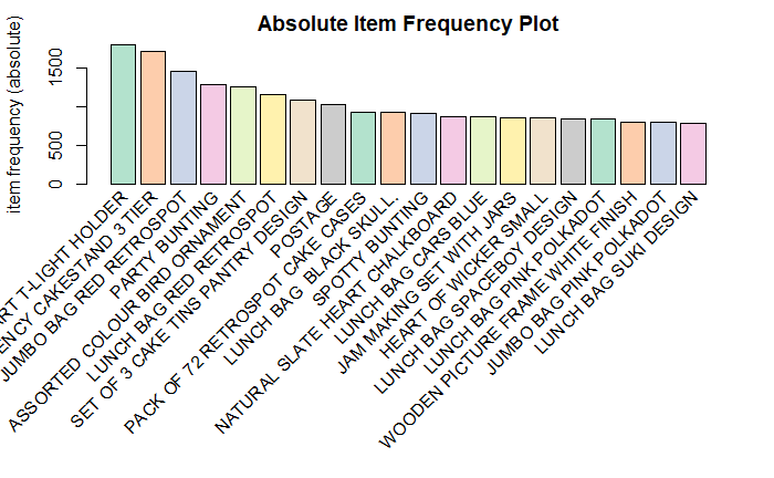

In 

itemFrequencyPlot(tr,topN=20,type="absolute")

first argument is the transaction object to be plotted that is tr. topN allows you to plot top N highest frequency items. type can be type="absolute" or type="relative". If absolute it will plot numeric frequencies of each item independently. If relative it will plot how many times these items have appeared as compared to others.

itemFrequencyPlot(tr,topN=20,type="relative",col=brewer.pal(8,'Pastel2'),main="Relative Item Frequency Plot")

This plot shows that 'WHITE HANGING HEART T-LIGHT HOLDER' and 'REGENCY CAKESTAND 3 TIER' have the most sales. So to increase the sale of 'SET OF 3 CAKE TINS PANTRY DESIGN' the retailer can put it near 'REGENCY CAKESTAND 3 TIER'.

You can explore other options for itemFrequencyPlot here.

Generating Rules!

Next step is to mine the rules using the APRIORI algorithm. The function apriori() is from package arules.

# Min Support as 0.001, confidence as 0.8.
association.rules <- apriori(tr, parameter = list(supp=0.001, conf=0.8,maxlen=10))

 Apriori

Parameter specification:
 confidence minval smax arem  aval originalSupport maxtime support minlen maxlen target
        0.8    0.1    1 none FALSE            TRUE       5   0.001      1     10  rules
   ext
 FALSE

Algorithmic control:
 filter tree heap memopt load sort verbose
    0.1 TRUE TRUE  FALSE TRUE    2    TRUE

Absolute minimum support count: 22

set item appearances ...[0 item(s)] done [0.00s].
set transactions ...[30066 item(s), 22191 transaction(s)] done [0.11s].
sorting and recoding items ... [2324 item(s)] done [0.02s].
creating transaction tree ... done [0.02s].
checking subsets of size 1 2 3 4 5 6 7 8 9 10

Mining stopped (maxlen reached). Only patterns up to a length of 10 returned!

 done [0.70s].
writing ... [49122 rule(s)] done [0.06s].
creating S4 object  ... done [0.06s]. 

set of 49122 rules

rule length distribution (lhs + rhs):sizes
    2     3     4     5     6     7     8     9    10
  105  2111  6854 16424 14855  6102  1937   613   121

   Min. 1st Qu.  Median    Mean 3rd Qu.    Max.
  2.000   5.000   5.000   5.499   6.000  10.000

summary of quality measures:
    support           confidence          lift             count       
 Min.   :0.001036   Min.   :0.8000   Min.   :  9.846   Min.   : 23.00  
 1st Qu.:0.001082   1st Qu.:0.8333   1st Qu.: 22.237   1st Qu.: 24.00  
 Median :0.001262   Median :0.8788   Median : 28.760   Median : 28.00  
 Mean   :0.001417   Mean   :0.8849   Mean   : 64.589   Mean   : 31.45  
 3rd Qu.:0.001532   3rd Qu.:0.9259   3rd Qu.: 69.200   3rd Qu.: 34.00  
 Max.   :0.015997   Max.   :1.0000   Max.   :715.839   Max.   :355.00  

mining info:
 data ntransactions support confidence
   tr         22191   0.001        0.8

The apriori will take tr as the transaction object on which mining is to be applied. parameter will allow you to set min_sup and min_confidence. The default values for parameter are minimum support of 0.1, the minimum confidence of 0.8, maximum of 10 items (maxlen).

summary(association.rules) shows the following:

• Parameter Specification: min_sup=0.001 and min_confidence=0.8 values with 10 items as max of items in a rule.

• Total number of rules: The set of 49122 rules

• Distribution of rule length: A length of 5 items has the most rules: 16424 and length of 2 items have the lowest number of rules:105

• Summary of Quality measures: Min and max values for Support, Confidence and, Lift.

• Information used for creating rules: The data, support, and confidence we provided to the algorithm.

Since there are 49122 rules, let's print only top 10:

inspect(association.rules[1:10])

     lhs                         rhs             support     confidence lift      count
[1]  {WOBBLY CHICKEN}         => {METAL}         0.001261773 1          443.82000 28   
[2]  {WOBBLY CHICKEN}         => {DECORATION}    0.001261773 1          443.82000 28   
[3]  {DECOUPAGE}              => {GREETING CARD} 0.001036456 1          389.31579 23   
[4]  {BILLBOARD FONTS DESIGN} => {WRAP}          0.001306836 1          715.83871 29   
[5]  {WOBBLY RABBIT}          => {METAL}         0.001532153 1          443.82000 34   
[6]  {WOBBLY RABBIT}          => {DECORATION}    0.001532153 1          443.82000 34   
[7]  {FUNK MONKEY}            => {ART LIGHTS}    0.001712406 1          583.97368 38   
[8]  {ART LIGHTS}             => {FUNK MONKEY}   0.001712406 1          583.97368 38   
[9]  {BLACK TEA}              => {SUGAR JARS}    0.002072912 1          238.61290 46   
[10] {BLACK TEA}              => {COFFEE}        0.002072912 1           69.34687 46 

Using the above output, you can make analysis such as:

• 100% of the customers who bought 'WOBBLY CHICKEN' also bought 'METAL'.

• 100% of the customers who bought 'BLACK TEA' also bought SUGAR 'JARS'.

Limiting the number and size of rules and

How can you limit the size and number of rules generated? You can do this by setting parameters in apriori. You set these parameters to adjust the number of rules you will get. If you want stronger rules, you can increase the value of conf and for more extended rules give higher value to maxlen.

shorter.association.rules <- apriori(tr, parameter = list(supp=0.001, conf=0.8,maxlen=3))

Removing redundant rules

You can remove rules that are subsets of larger rules. Use the code below to remove such rules:

subset.rules <- which(colSums(is.subset(association.rules, association.rules)) > 1) # get subset rules in vector
length(subset.rules)  #> 3913

[1] 44014

subset.association.rules. <- association.rules[-subset.rules] # remove subset rules.

• which() returns the position of elements in the vector for which value is TRUE.

• colSums() forms a row and column sums for dataframes and numeric arrays.

• is.subset() Determines if elements of one vector contain all the elements of other

Finding Rules related to given items

Sometimes, you want to work on a specific product. If you want to find out what causes influence on the purchase of item X you can use appearance option in the apriori command. appearance gives us options to set LHS (IF part) and RHS (THEN part) of the rule.

For example, to find what customers buy before buying 'METAL' run the following line of code:

metal.association.rules <- apriori(tr, parameter = list(supp=0.001, conf=0.8),appearance = list(default="lhs",rhs="METAL"))

Apriori

Parameter specification:
 confidence minval smax arem  aval originalSupport maxtime support minlen maxlen target
        0.8    0.1    1 none FALSE            TRUE       5   0.001      1     10  rules
   ext
 FALSE

Algorithmic control:
 filter tree heap memopt load sort verbose
    0.1 TRUE TRUE  FALSE TRUE    2    TRUE

Absolute minimum support count: 22

set item appearances ...[1 item(s)] done [0.00s].
set transactions ...[30066 item(s), 22191 transaction(s)] done [0.21s].
sorting and recoding items ... [2324 item(s)] done [0.02s].
creating transaction tree ... done [0.02s].
checking subsets of size 1 2 3 4 5 6 7 8 9 10

Mining stopped (maxlen reached). Only patterns up to a length of 10 returned!

 done [0.63s].
writing ... [5 rule(s)] done [0.07s].
creating S4 object  ... done [0.02s]. 

# Here lhs=METAL because you want to find out the probability of that in how many customers buy METAL along with other items
inspect(head(metal.association.rules))

    lhs                            rhs     support     confidence lift   count
[1] {WOBBLY CHICKEN}            => {METAL} 0.001261773 1          443.82 28   
[2] {WOBBLY RABBIT}             => {METAL} 0.001532153 1          443.82 34   
[3] {DECORATION}                => {METAL} 0.002253166 1          443.82 50   
[4] {DECORATION,WOBBLY CHICKEN} => {METAL} 0.001261773 1          443.82 28   
[5] {DECORATION,WOBBLY RABBIT}  => {METAL} 0.001532153 1          443.82 34 

Similarly, to find the answer to the question Customers who bought METAL also bought.... you will keep METAL on lhs:

metal.association.rules <- apriori(tr, parameter = list(supp=0.001, conf=0.8),appearance = list(lhs="METAL",default="rhs"))

Apriori

Parameter specification:
 confidence minval smax arem  aval originalSupport maxtime support minlen maxlen target
        0.8    0.1    1 none FALSE            TRUE       5   0.001      1     10  rules
   ext
 FALSE

Algorithmic control:
 filter tree heap memopt load sort verbose
    0.1 TRUE TRUE  FALSE TRUE    2    TRUE

Absolute minimum support count: 22

set item appearances ...[1 item(s)] done [0.00s].
set transactions ...[30066 item(s), 22191 transaction(s)] done [0.10s].
sorting and recoding items ... [2324 item(s)] done [0.02s].
creating transaction tree ... done [0.02s].
checking subsets of size 1 2 done [0.01s].
writing ... [1 rule(s)] done [0.00s].
creating S4 object  ... done [0.01s].

# Here lhs=METAL because you want to find out the probability of that in how many customers buy METAL along with other items
inspect(head(metal.association.rules))

    lhs        rhs          support     confidence lift   count
[1] {METAL} => {DECORATION} 0.002253166 1          443.82 50 

Visualizing Association Rules

Since there will be hundreds or thousands of rules generated based on data, you need a couple of ways to present your findings. ItemFrequencyPlot has already been discussed above which is also a great way to get top sold items.

Here the following visualization will be discussed:

• Scatter-Plot
• Interactive Scatter-plot
• Individual Rule Representation

Scatter-Plot

A straight-forward visualization of association rules is to use a scatter plot using plot() of the arulesViz package. It uses Support and Confidence on the axes. In addition, third measure Lift is used by default to color (grey levels) of the points.

# Filter rules with confidence greater than 0.4 or 40%
subRules<-association.rules[quality(association.rules)$confidence>0.4]
#Plot SubRules
plot(subRules)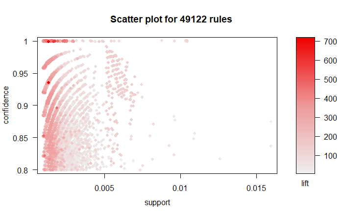

The above plot shows that rules with high lift have low support. You can use the following options for the plot:

plot(rulesObject, measure, shading, method)

• rulesObject: the rules object to be plotted

• measure: Measures for rule interestingness. Can be Support, Confidence, lift or combination of these depending upon method value.

• shading: Measure used to color points (Support, Confidence, lift). The default is Lift.

• method: Visualization method to be used (scatterplot, two-key plot, matrix3D).

plot(subRules,method="two-key plot")

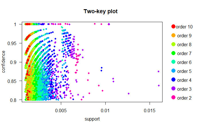
The two-key plot uses support and confidence on x and y-axis respectively. It uses order for coloring. The order is the number of items in the rule.

Interactive Scatter-Plot

An amazing interactive plot can be used to present your rules that use arulesViz and plotly. You can hover over each rule and view all quality measures (support, confidence and lift).

plotly_arules(subRules)

'plotly_arules' is deprecated.
Use 'plot' instead.
See help("Deprecated")plot: Too many rules supplied. Only plotting the best 1000 rules using measure lift (change parameter max if needed)To reduce overplotting, jitter is added! Use jitter = 0 to prevent jitter.

Graph-Based Visualizations

Graph-based techniques visualize association rules using vertices and edges where vertices are labeled with item names, and item sets or rules are represented as a second set of vertices. Items are connected with item-sets/rules using directed arrows. Arrows pointing from items to rule vertices indicate LHS items and an arrow from a rule to an item indicates the RHS. The size and color of vertices often represent interest measures.

Graph plots are a great way to visualize rules but tend to become congested as the number of rules increases. So it is better to visualize less number of rules with graph-based visualizations.

Let's select 10 rules from subRules having the highest confidence.

top10subRules <- head(subRules, n = 10, by = "confidence")

Now, plot an interactive graph:

Note: You can make all your plots interactive using engine=htmlwidget parameter in plot

plot(top10subRules, method = "graph",  engine = "htmlwidget")

From arulesViz graphs for sets of association rules can be exported in the GraphML format or as a Graphviz dot-file to be explored in tools like Gephi. For example, the 1000 rules with the highest lift are exported by:

saveAsGraph(head(subRules, n = 1000, by = "lift"), file = "rules.graphml")

Individual Rule Representation

This representation is also called as Parallel Coordinates Plot. It is useful to visualized which products along with which items cause what kind of sales.

As mentioned above, the RHS is the Consequent or the item we propose the customer will buy; the positions are in the LHS where 2 is the most recent addition to our basket and 1 is the item we previously had.

# Filter top 20 rules with highest lift
subRules2<-head(subRules, n=20, by="lift")
plot(subRules2, method="paracoord")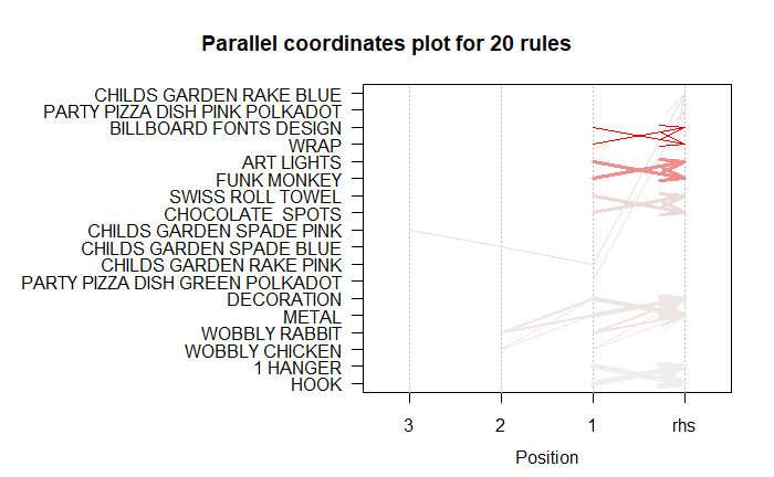

Look at the topmost arrow. It shows that when I have 'CHILDS GARDEN SPADE PINK' and 'CHILDS GARDEN RAKE PINK' in my shopping cart, I am likely to buy 'CHILDS GARDEN RAKE BLUE' along with these as well.

Conclusion

Congratulations! You have learned APRIORI, one of the most frequently used algorithms in data mining. You have learned all about Association Rule Mining, its applications, and its applications in retailing called as Market Basket Analysis. You are also now capable of implementing Market Basket Analysis in R and presenting your association rules with some great plots! Happy learning!

References:

1. https://datascienceplus.com/a-gentle-introduction-on-market-basket-analysis%E2%80%8A-%E2%80%8Aassociation-rules/

2. https://en.wikipedia.org/wiki/Sparse_matrix

3. https://cran.r-project.org/web/packages/arulesViz/vignettes/arulesViz.pdf

If you would like to learn more about R, take DataCamp's Importing and Managing Financial Data in R course.