PyTorch Lightning: A Comprehensive Hands-On Tutorial

PyTorch Lightning is a massively popular wrapper for PyTorch that makes it easy to develop and train deep learning models. It eliminates boilerplate code for training loops and complex setups, which is cumbersome for many developers, and allows you to focus on the core model and experiment logic.

Features of PyTorch Lightning:

• Simplifies the codebase through minimal boilerplate code.
• Offers multi-GPU and distributed training for scalability.
• Integrates with PyTorch.
• Encourages organized and modular code.
• Simplifies complex setups like mixed precision tuning and distributed training.
• Offers built-in features for checkpoints, logs, and experiment tracking.

We will see the benefits of these features as we go through real-world examples in this tutorial. Let’s get started!

Setting Up a PyTorch Lightning Environment

Before we start coding, let’s set up our environment, download a dataset, and define the problem statement for our example project.

1. Environment setup and installation

We will start by creating a Conda environment:

$ conda create -n lightning python=3.9 -y
$ conda activate lightning

After activating the environment, we install lightning and a few other necessary libraries:

$ pip install lightning
$ pip install ipykernel

ipykernel lets us add our new Conda environment to Jupyter as a kernel:

$ ipython kernel install --user --name=lightning

lightning automatically installs classic PyTorch, so the following code must work:

import lightning as L
import torch

print("Lightning version:", L.__version__)
print("Torch version:", torch.__version__)
print("CUDA is available:", torch.cuda.is_available())

Lightning version: 2.3.2
Torch version: 2.1.2+cu121
CUDA is available: True

It is recommended that you run the code examples on a machine with a GPU. The PyTorch documentation provides installation options.

This tutorial includes a PyTorch refresher section, but if you are completely new, here are some relevant resources:

• Introduction to PyTorch Tutorial
• Introduction to Deep Learning In PyTorch
• Intermediate Deep Learning With PyTorch
• Deep Learning For Images With PyTorch
• Deep Learning in Python Skill Track

Now, let’s import some modules:

import torch
import torch.nn as nn
import torch.nn.functional as F
import torch.optim as optim
import lightning as L
from torch.utils.data import DataLoader
from torchvision import datasets, transforms
from lightning.pytorch.callbacks import ModelCheckpoint
from lightning.pytorch.loggers.tensorboard import TensorBoardLogger
from lightning.pytorch.callbacks.early_stopping import EarlyStopping

These imports give us access to PyTorch Lightning’s core functionality (L), PyTorch's neural network modules (nn), and various utility functions.

It is also a good practice to set random seed for reproducibility:

L.seed_everything(1121218)

Let’s also set a few hyperparameters that rarely change for the rest of the tutorial:

num_epochs = 10
batch_size = 64
learning_rate = 0.001

Note on terminology: At the time of writing, the PyTorch Lightning Python package has two different names. In the past, it was named pytorch_lightning and imported as pl. After the company behind it was rebranded to Lightning AI, the package name was changed to lightning. Even though the old version still gets updates and downloads, it is recommended to use lightning.

2. Problem statement and downloading a dataset

We will see how to leverage PyTorch Lightning through a classic multi-class classification problem using the CIFAR10 dataset.

The dataset consists of 60 thousand 32x32 color images in 10 classes, with 6000 images per class.

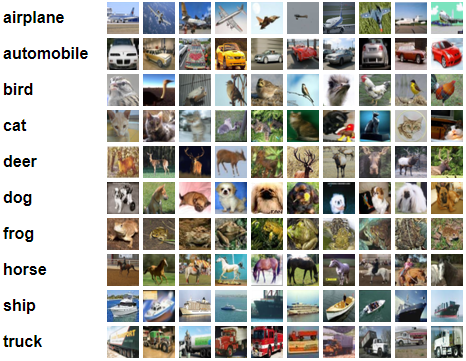
CIFAR10 dataset overview.

You can download the data as a tar.gz file, but using it would involve several extraction and processing steps. Instead, we can use the datasets.CIFAR10 function from torchvision:

from torchvision import datasets, transforms

# Load CIFAR-10 dataset
train_dataset = datasets.CIFAR10(
   root="./data", train=True, download=True, transform=transform_train
)
val_dataset = datasets.CIFAR10(
   root="./data", train=False, download=True, transform=transform_test
)

Here is the breakdown of the arguments passed to the datasets.CIFAR10() function:

• root: Specifies the location where to download the dataset.
• train: Specifies whether to download the train or test set
• download: Whether to download the dataset from source. If it already exists, it is verified against the source.

The transform argument expects a transformation pipeline defined using the Compose class from transforms. Here are transform_train and transform_test pipelines that we pass to the transform argument:

# Data augmentation and normalization for training
transform_train = transforms.Compose(
   [
       transforms.RandomCrop(32, padding=4),
       transforms.RandomHorizontalFlip(),
       transforms.ToTensor(),
       transforms.Normalize((0.5, 0.5, 0.5), (0.5, 0.5, 0.5)),
   ],
)
transform_test = transforms.Compose(
   [transforms.ToTensor(), transforms.Normalize((0.5, 0.5, 0.5), (0.5, 0.5, 0.5))]
)

People familiar with PyTorch know that these pipelines perform data augmentation in which dataset size is artificially increased through random transformations. 

In the code above, we do the following:

• Cropping (requires the image size to be specified, 32x32 in this case).
• Horizontal flipping.
• Converting to a tensor data type, which is required for PyTorch.
• Normalization of each color channel of images.

Data augmentation doesn’t create new images but duplicates the existing ones from different “angles” or “lenses” to simulate various real-world conditions. It is an advantageous technique for deep learning models.

Once the dataset is downloaded, you will have a data directory with the following structure:

./data/cifar-10-batches-py/
├── batches.meta
├── data_batch_1
├── data_batch_2
├── data_batch_3
├── data_batch_4
├── data_batch_5
├── readme.html
└── test_batch

The data_batch_* and test_batch are Python pickle files containing the images and labels. Each batch contains a dictionary with the following elements:

• data: A 10000x3072 numpy array of uint8. Each row is a 32x32 color image with 3 channels (RGB).
• labels: A list of 10000 numbers in the range 0-9, representing the class of each image.

The datasets.CIFAR10 function unpickles these files and presents them in a format compatible with PyTorch DataLoaders:

train_loader = DataLoader(
   train_dataset, batch_size=batch_size, shuffle=True, num_workers=8
)
test_loader = DataLoader(
   test_dataset, batch_size=batch_size, shuffle=False, num_workers=8
)

DataLoader classes are essential utilities for data preparation and model training. They can:

• Handle data loading, preprocessing, and batching simultaneously.
• Support multi-threading to maximize CPU utilization (num_workers).
• Minimize training bottlenecks.
• Shuffle the data after every epoch (shuffle).
• Be highly efficient for large datasets.

Whether you use classic Torch or the new Lightning, the data loading and preparation steps stay mostly the same, as both use PyTorch Dataset or DataLoader objects.

Now, we will train a CNN model using both frameworks to see what advantages Lightning has over classic PyTorch.

Classic PyTorch Workflow Revisited

First, let’s briefly review how to train a CNN using classic PyTorch. Then, we will re-execute using Lightning.

1. Defining the model architecture

After creating data loaders, the first step is defining the model architecture using the nn.Module class:

class CIFAR10CNN(nn.Module):
   def __init__(self):
       super(CIFAR10CNN, self).__init__()
       self.conv1 = nn.Conv2d(3, 32, 3, padding=1)
       self.conv2 = nn.Conv2d(32, 64, 3, padding=1)
       self.conv3 = nn.Conv2d(64, 64, 3, padding=1)
       self.pool = nn.MaxPool2d(2, 2)
       self.fc1 = nn.Linear(64 * 4 * 4, 512)
       self.fc2 = nn.Linear(512, 10)
   def forward(self, x):
       x = self.pool(torch.relu(self.conv1(x)))
       x = self.pool(torch.relu(self.conv2(x)))
       x = self.pool(torch.relu(self.conv3(x)))
       x = x.view(-1, 64 * 4 * 4)
       x = torch.relu(self.fc1(x))
       x = self.fc2(x)
       return x

By inheriting from the PyTorch nn.Module (neural networks), we can create complex and flexible architectures. In the code above, we create three convolution layers followed by max pooling and two linear layers. The forward() method defines the ordering of these layers and adds activation functions.

The model architecture syntax stays the same for Lightning except for one detail, which we will see later in the tutorial. Every subsequent step changes as Lightning introduces enhanced syntax that reduces boilerplate code.

2. Writing training and validation loops

The next part is writing the dreaded training and validation loop, which requires you to memorize the order of the following steps:

• Initializing the model, loss function, and optimizers.
• Device management (CPU vs. GPU).
• Training steps: forward pass, loss computation, backpropagation, and optimization.
• Validation steps: computing accuracy and loss.
• Tensorboard logging.
• Model saving.

The result is a code snippet so large that requires a few dozen practice sessions to thoroughly memorize. I pasted the code in this GitHub gist to save space; below are the first few lines:

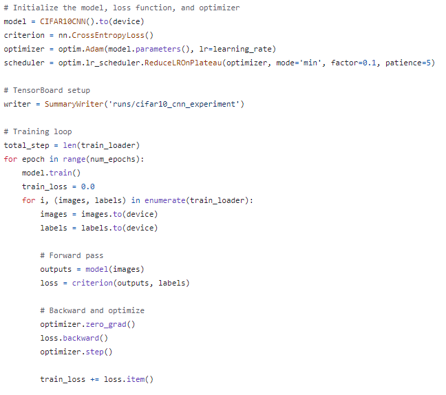
The first few lines of code of a classic PyTorch workflow.

Here are a few other details to note about the code example above:

• There’s manual switching between training and validation modes.
• There’s a manual specification of gradient computation.
• The usage of the inferior SummaryWriter class for logging.
• There’s a learning rate scheduler.

PyTorch Lightning Workflow

Now, let’s see how PyTorch Lightning compares to the classic PyTorch workflow.

1. Defining the model architecture with the LightningModule class

Defining model architecture in Lightning is almost the same as in pure PyTorch:

class CIFAR10CNN(L.LightningModule):
   def __init__(self):
       super().__init__()
       self.conv1 = nn.Conv2d(3, 32, 3, padding=1)
       self.conv2 = nn.Conv2d(32, 64, 3, padding=1)
       self.conv3 = nn.Conv2d(64, 64, 3, padding=1)
       self.pool = nn.MaxPool2d(2, 2)
       self.fc1 = nn.Linear(64 * 4 * 4, 512)
       self.fc2 = nn.Linear(512, 10)
   def forward(self, x):
       x = self.pool(F.relu(self.conv1(x)))
       x = self.pool(F.relu(self.conv2(x)))
       x = self.pool(F.relu(self.conv3(x)))
       x = x.view(-1, 64 * 4 * 4)
       x = F.relu(self.fc1(x))
       x = self.fc2(x)
       return x

The only difference is that we inherit from the LightningModule class, not from the nn.Module.

The LightningModule is an extension of the nn.Module class. It combines the training, validation, testing, prediction, and optimization steps of the PyTorch workflow into a single interface without loops. 

When you start using LightningModule, the PyTorch code isn't abstracted; it’s organized into six sections:

• Initialization (__init__ and setup() methods).
• Train loop (training_step() method).
• Validation loop (validation_step() method).
• Test loop (test_step() method).
• Prediction loop (prediction_step() method).
• Optimizers and LR schedulers (configure_optimizers()).

We’ve already seen the initialization part. Let’s move on to the training step.

2. Writing a training step

To activate a training loop, we override the training_step() method of our model class:

# Add the method inside the class
def training_step(self, batch, batch_idx):
   x, y = batch
   y_hat = self(x)
   loss = F.cross_entropy(y_hat, y)
   self.log('train_loss', loss)
   return loss

This method collapses the entire training loop into a few lines of code. First, we extract the feature and target arrays from the current batch, which is provided by a data loader. Then, we run a forward pass self(x) and compute the loss. Then, we simply log the training loss using the built-in Lightning logger function self.log().

You can also log other metrics like training accuracy inside this method:

def training_step(self, batch, batch_idx):
   x, y = batch
   y_hat = self(x)
  
   loss = F.cross_entropy(y_hat, y)
   acc = (y_hat.argmax(1) == y).float().mean()
  
   self.log("train_loss", loss)
   self.log("train_acc", acc)
   return loss

The log() method automatically reduces the metrics calculation to the epoch level. It has additional parameters if you want custom logs:

# Log the loss at each training step and epoch, create a progress bar
self.log("train_loss", loss, on_step=True, on_epoch=True, prog_bar=True, logger=True)

In the end, you just have to remember to return the computed loss (only the loss, not other metrics). To learn more about the training step, visit the Lightning AI documentation page.

3. Writing validation and test steps

The validation and test steps are very similar to the training step:

def validation_step(self, batch, batch_idx):
   x, y = batch
   y_hat = self(x)
   loss = F.cross_entropy(y_hat, y)
   acc = (y_hat.argmax(1) == y).float().mean()
   self.log('val_loss', loss)
   self.log('val_acc', acc)
def test_step(self, batch, batch_idx):
   x, y = batch
   y_hat = self(x)
   loss = F.cross_entropy(y_hat, y)
   acc = (y_hat.argmax(1) == y).float().mean()
   self.log('test_loss', loss)
   self.log('test_acc', acc)

The only difference is that you don’t return the computed metrics. Lightning automatically assigns the correct data loaders to the validation and test steps and creates the loops under the hood.

Even though validation_step() and test_step() look the same, they have a key distinction:

• validation_step() goes into action during training.
• test_step() does so during testing, or in other words, when you call the trainer object's .test() method. We will see an example later in the tutorial.

See the validation and testing sections of the Lightning AI documentation for more details.

4. Configuring optimization and LR schedulers

To define an optimizer and a learning rate scheduler, we need to override the configure_optimizers() method of our class:

def configure_optimizers(self):
   optimizer = torch.optim.Adam(self.parameters(), lr=1e-3)
   scheduler = torch.optim.lr_scheduler.ReduceLROnPlateau(
       optimizer, mode="min", factor=0.1, patience=5
   )
  
   return {
       "optimizer": optimizer,
       "lr_scheduler": {
           "scheduler": scheduler,
           "monitor": "val_loss",
       },
   }

Above, we create an Adam optimizer, passing in the hyperparameters and the learning rate. We also define a ReduceLROnPlateau scheduler to reduce the learning rate when validation loss plateaus.

Both of these objects must be returned in one of the following ways:

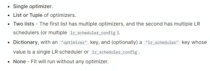
Returning a dictionary of objects is the most flexible option, as it allows defining schedulers that require extra arguments. For more details, refer to this section of the Lightning AI documentation.

5. Defining callbacks and loggers

Our model class, CIFAR10CNN is finally ready. Before we start training, let's set up a couple of helpful callbacks and a logger. The first one is a model checkpoint callback:

checkpoint_callback = ModelCheckpoint(
   dirpath="checkpoints",
   monitor="val_loss",
   filename="cifar10-{epoch:02d}-{val_loss:.2f}-{val_acc:.2f}",
   save_top_k=3,
   mode="min",
)

The ModelCheckpoint class is a powerful callback to periodically save the model while monitoring a given metric. Each model checkpoint is logged to the provided dirpath with the metric specified in monitor.

The filename represents the name for each checkpoint file. By default, they are set to {epoch}-{step} style, but you can use any custom filename with formatting options. For example, the above callback creates filenames with:

• Epoch numbers are zero-padded to two digits.
• Validation loss and accuracy as floating point numbers with two decimal places.

The save_top_k controls how many checkpoint files are saved with the following conditions:

• save_top_k == 0, no models are saved.
• save_top_k == -1, all models are saved.
• save_top_k >= 2, top K models are saved.

We will also define a TensorBoardLogger:

logger = TensorBoardLogger(save_dir="lightning_logs", name="cifar10_cnn")

The class reports model training progress to local or remote file systems in TensorBoard format. The final object (callback) we define is EarlyStopping:

early_stopping = EarlyStopping(monitor="val_loss", patience=5, mode="min", verbose=False)

“Early stopping” is a popular technique to control the training of models that use optimization functions. By enabling it, Lightning can stop training if the validation loss hasn’t been improving for a certain number of epochs.

Here’s the meaning of each argument passed to the EarlyStopping class

• monitor: The metric to watch.
• patience: The number of epochs to wait before stopping the training if the metric hasn't been improving
• mode: When set to min, training stops when the metric has stopped decreasing. In max, it will stop when the metric has stopped increasing.

6. Creating a Trainer class

Once we have organized everything into a LightningModule class and defined the loggers and callbacks, a Trainer class automates everything else.

Here is its basic syntax:

# DON'T RUN THIS CODE JUST YET
# Initialize the model
model = CIFAR10CNN()
# Initialize the trainer
trainer = L.Trainer()
trainer.fit(model, train_loader, test_loader)

Under the hood, the trainer handles all loop details for you:

• Automatically enabling and disabling gradients.
• Running the training, validation, and test data loaders.
• Calling the callbacks at the appropriate times.
• Assigning batches and computations to the correct devices.

It also accepts several training details as arguments:

# Initialize the Trainer
trainer = L.Trainer(
   max_epochs=50,
   callbacks=[checkpoint_callback, early_stopping],
   logger=logger,
   accelerator="gpu" if torch.cuda.is_available() else "cpu",
   devices="auto",
)
GPU available: True (cuda), used: True
TPU available: False, using: 0 TPU cores
HPU available: False, using: 0 HPUs

In the code above, we pass the number of epochs to train, the callbacks, the logger, and whether to use GPU acceleration.

7. Running and testing the model

Once the trainer is ready, we can finally call .fit() on the model class and the data loaders (find the full code of the previous sections here):

# Train and test the model

trainer.fit(model, train_loader, test_loader)

trainer.test(model, test_loader)

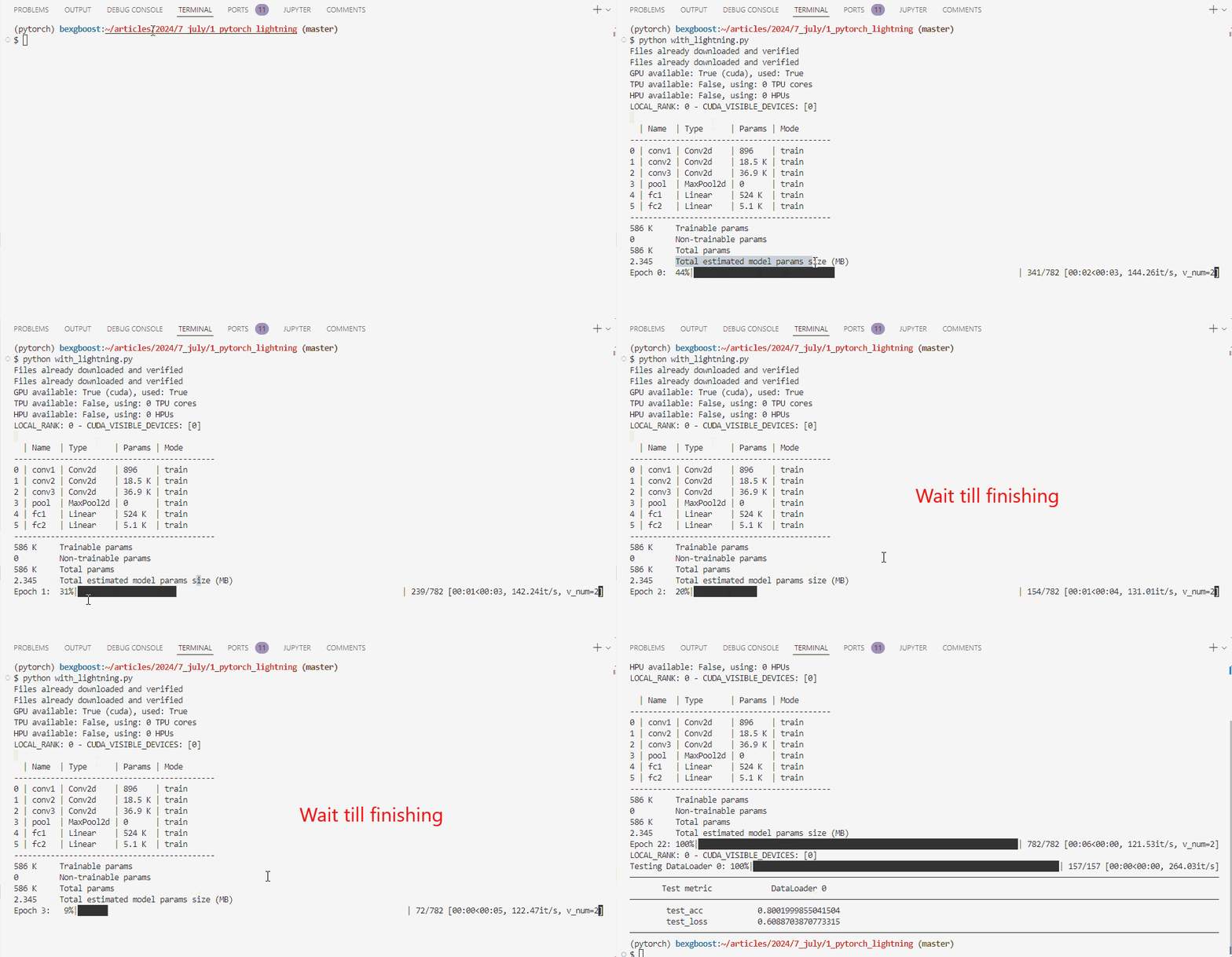
Training and testing the PyTorch Lightning model.

After training, we can see that our test accuracy was 80% — not bad considering we haven’t given the model architecture much thought. 

Let’s explore our working directory:

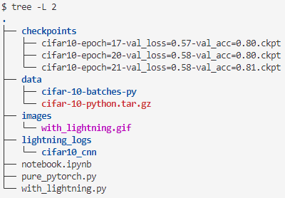
PyTorch Lightning project working directory.

The checkpoints and lightning_logs directories show that everything worked as expected.

8. Summary of the PyTorch Lightning training workflow

Let’s take a step back and summarize the steps we implemented on a higher level:

1. Installation and setup.
2. Downloading the dataset manually or through the dataset package of torchvision.
3. Creating training, validation, and testing data loaders with transformations applied.
4. Organizing our code into a LightningModule class:
• Defining the initialization.
• Defining the training, validation, and (optional) test steps.
• Defining optimizers and learning rate schedulers.
5. Defining callbacks and loggers.
6. Creating a Trainer class.
7. Initializing the model class.
8. Fitting and testing the model.

These steps can serve as a rough blueprint for your other projects. They are much more straightforward than memorizing the order of training and validation loops.

PyTorch Lightning Data Modules

My favorite aspect of Lightning is its custom data modules. In traditional PyTorch code, data operations are scattered across different files or, worse, different mediums (both scripts and the terminal). This makes it impossible to share and reuse the exact steps you took for the dataset to transform from state A to state Z.

Data modules elegantly encompass all these details into a single class. They have the following methods,  which return processed train, validation, testing, and prediction data loaders:

• prepare_data()
• setup()
• train_dataloader()
• val_dataloader()
• test_dataloader()
• predict_dataloader()
• teardown()

prepare_data() ensures that the data is downloaded and saved using only a single process. A plain script run with distributed settings (on multiple processes) may result in corrupted data. As prepare_data() runs, setup() waits for its full execution. Then, it can perform transformations and splitting using multiple processes on a CPU or GPU.

Since prepare_data() runs on a single process, you shouldn't set the class state here. In other words, don't use the self keyword inside prepare_data() because a variable is defined as self.x = 1 won't be available to different processes.

Now, let’s encapsulate all operations we performed on the CIFAR10 dataset into a single data module:

class CIFAR10DataModule(L.LightningDataModule):
   def __init__(self, data_dir = "./data", batch_size = 64):
       # Define any custom user-defined parameters
       super().__init__()
       self.data_dir = data_dir
       self.batch_size = batch_size
       self.transform_train = transforms.Compose(
           [
               transforms.RandomCrop(32, padding=4),
               transforms.RandomHorizontalFlip(),
               transforms.ToTensor(),
               transforms.Normalize((0.5, 0.5, 0.5), (0.5, 0.5, 0.5)),
           ],
       )
       self.transform_test = transforms.Compose(
           [transforms.ToTensor(), transforms.Normalize((0.5, 0.5, 0.5), (0.5, 0.5, 0.5))]
       )

First, we create a class that inherits from the LightningDataModule class. Then, we override the initialization method and define a couple of variables. We also initialize the transformation pipelines we want to perform on the data.

Next, we override the prepare_data() method:

def prepare_data(self):
   # Download the data
   datasets.CIFAR10(self.data_dir, train=True, download=True)
   datasets.CIFAR10(self.data_dir, train=False, download=True)

The method downloads and saves the data to the data_dir path.

The next step is overriding the setup() method to load the data from the downloaded path and applying the transformation steps:

def setup(self, stage=None):
   if stage == 'fit' or stage is None:
       self.cifar_train = datasets.CIFAR10(self.data_dir, train=True, transform=self.transform)
       self.cifar_val = datasets.CIFAR10(self.data_dir, train=False, transform=self.transform)
   if stage == 'test' or stage is None:
       self.cifar_test = datasets.CIFAR10(self.data_dir, train=False, transform=self.transform)

The setup() must accept one argument for the stage to apply stage-specific transformations. Above, we are loading different parts of the CIFAR10 dataset for various stages of model development.

Finally, we override three more methods to return the processed datasets as data loaders:

def train_dataloader(self):
       return DataLoader(self.cifar_train, batch_size=self.batch_size, shuffle=True)
def val_dataloader(self):
   return DataLoader(self.cifar_val, batch_size=self.batch_size)
def test_dataloader(self):
   return DataLoader(self.cifar_test, batch_size=self.batch_size)

Using this data module is straightforward now:

# Initialize the data module
data_module = CIFAR10DataModule()
# Initialize the model and trainer
model = CIFAR10CNN()
trainer = Trainer(...)
# Fit the model
trainer.fit(model, data_module)
# Test the model
trainer.test(model, data_module)

Using data modules offers several benefits:

• Simplicity: The CIFAR10 dataset is handled easily with built-in torchvision functions.
• Modularity: You can swap out datasets by creating new data modules without changing the model code.
• Reproducibility: Data processing steps are clearly defined and reproducible.
• Separation: Data handling is separated from model logic, leading to cleaner code.

For datasets requiring complex and lengthy data modules, consider creating a separate script and then importing it from your training script.

PyTorch Lightning Best Practices and Tips

In this section, we will outline a few debugging, optimization and organization tips.

Debugging strategies

• Use the fast_dev_run option. This will run only one batch of training, validation, and testing to catch any errors before running all epochs:

trainer = L.Trainer(fast_dev_run=True)

• Use the overfit_batches parameter to check if your model can overfit on a small subset of data. A good practice in deep learning is to create a model that can overfit the data first, then regularize:

trainer = L.Trainer(overfit_batches=100)

Performance optimization

• Enable automatic mixed precision tuning for faster training on modern GPUs:

trainer = L.Trainer(precision=16)

• Use gradient accumulation when you are limited by GPU size but need larger batch sizes. This accumulates gradients over four batches before updating weights:

trainer = L.Trainer(accumulate_grad_batches=4)

Code organization

• Separate model architecture from training logic. Keep your LightningModule focused on the model architecture and training process. Move data-related operations to the data module.

• Use config files. Store hyperparameters and model configurations in separate YAML files:

from omegaconf import OmegaConf

config = OmegaConf.load('config.yaml')
model = MyModel(config.model)
trainer = L.Trainer(**config.trainer)

• Implement custom callbacks. Use callbacks for non-essential logic to keep your LightningModule clean:

class MyCallback(L.Callback):
   def on_train_epoch_end(self, trainer, pl_module):
       # Custom logic here
  trainer = L.Trainer(callbacks=[MyCallback()])

• Utilize Lightning CLI to streamline experiment configuration:

from pytorch_lightning.cli import LightningCLI

cli = LightningCLI(MyModel, MyDataModule)

• Version control your experiments using tools like MLflow or Weights & Biases to track your experiments:

from pytorch_lightning.loggers import MLFlowLogger

logger = MLFlowLogger(experiment_name="my_experiment")
trainer = pl.Trainer(logger=logger)

• Implement unit tests for individual components of your pipeline:

def test_model_output():
   model = MyModel()
   x = torch.randn(1, 3, 224, 224)
   output = model(x)
   assert output.shape == torch.Size([1, 10])

Conclusion and Further Resources

In this tutorial, we have covered the fundamentals of using PyTorch Lightning in deep learning. Through the example of training a CNN on the CIFAR10 dataset, we have learned how to:

• Create LightningModule classes to organize model architecture code.
• Create Trainer classes to collapse long training loops into a few lines of code.
• Define callbacks and loggers to add to the training process.
• Modularize data handling using LightDataModule classes.
• Improve your code through best practices and tips.

For the most up-to-date information, regularly visit the Lightning AI documentation. Here are some other related resources to accelerate your learning:

• Deep Learning on Rails with PyTorch Lightning
• Top 26 Python Libraries for Data Science in 2024
• A Comprehensive Guide to Building a Transformer Model with PyTorch