Isolation Forest Guide: Explanation and Python Implementation

I recently got a text from my bank: 

“We placed a hold on your card. Is transaction for [amount] at [vendor] yours?” 

Thankfully, it was just me online shopping at an unreasonable hour, but it got me thinking… how does the bank flag suspicious transactions amongst all the hundreds of thousands it processes a day?

Identifying fraud is a specific case of a wider problem in machine learning (ML) called anomaly detection. While there are many methods to solve this problem, we’ll focus in this blog on one of the most popular: Isolation Forests.

Anomaly Detection in Practice

Fighting fraud, defending networks, finding outliers, and flagging faulty equipment may all seem like different problems. However, they share a common trait—no clear labels or definitions of what constitutes an anomaly. In many cases, anomalies are rare and subtle, making them difficult to identify amidst vast amounts of normal data.

One way to develop anomaly detection systems is to use predictive ML. For example, we could collect fraudulent transactions. Then, using features like transaction amount, time, location, and type of merchant, we can build a model that distinguishes these from normal transactions. The problem is this approach will only allow us to detect cases of fraud similar to the ones we’ve seen in the past. 

Fraudsters will often change their strategies and attempt new ways of committing fraud. Many of these strategies will be completely unexpected. This is why unsupervised methods are often used to detect anomalies. They work by comparing all transactions and identifying ones that have unusual feature values. Importantly, this means we do not have to label any transactions beforehand.

Fraud is not the only behavior that is difficult to classify. In manufacturing, machines can fail at any time in a variety of unexpected ways. In cyber security, novel attacks are constantly being found and patched. In medicine, rare health issues can be hidden among many test results.  The applications are endless, so let’s see how one unsupervised approach to detecting these anomalies works. 

What Is an Isolation Forest?

If you didn’t guess by the name, Isolation Forests are a tree-based method. They are similar to Random Forests. However, the basic building blocks are different.

A Random Forest uses decision trees created using splits based on gini impurity. This requires a target variable so, instead, Isolation Forests use Isolation Trees. The method uses a collection of these trees to calculate anomaly scores for each instance. 

Isolation Trees

It is worth understanding how this basic building block works before we calculate anomaly scores. Let’s say we are trying to detect fraudulent transactions. To keep things simple, we will evaluate 1000 transactions (instances) and consider two variables from our dataset: the amount (x₁) and time of day (x₂) of a transaction.

To create an Isolation Tree, we start with all or a sample of instances in the root node. In Figure 1 below, you can see we have a sample of 256 instances (more on that number later).

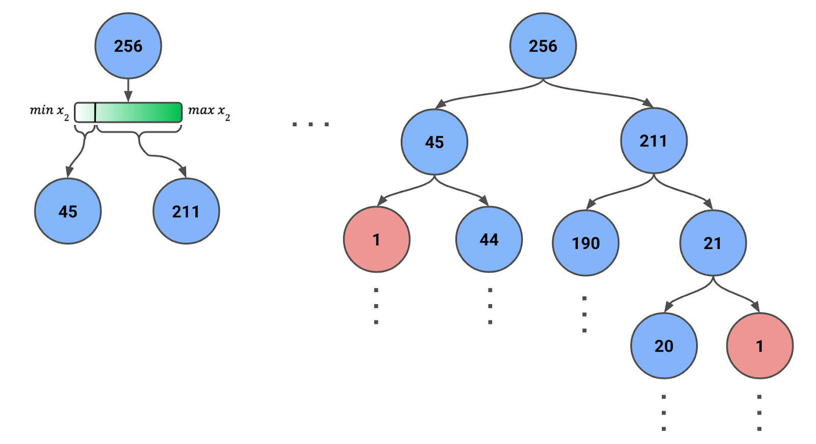
Figure 1: Isolation Tree created using recursive random splits. The number of instances in each node is given.

We then:

1. Randomly select a feature (either x₁ or x₂). 
2. Randomly select a split value within the range of the selected feature for the instances currently in the node.
3. Partition the data into two child nodes based on the split value.
4. Repeat the process recursively for each child node until one of the following conditions is met:
1. Each leaf node has only one instance.
2. A predefined maximum depth is reached.

Note that the feature’s range will change for each step. That is, we use the feature's minimum and maximum values for the node's instances. This dynamic adjustment ensures that splits are meaningful and that nodes do not end up with zero instances.

Figure 2 below gives us some intuition for why this process isolates outliers. Instances A, B, and C seem different from the other transactions.

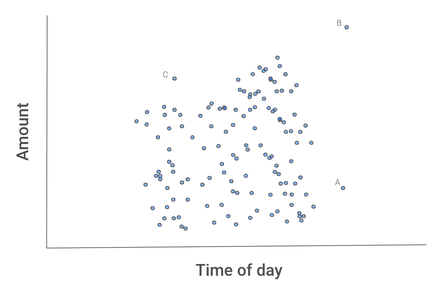
Figure 2: Scatter plot of transactions 

B will likely be isolated first as it can be separated from the other transactions using one split from either feature.

A would take one split from x₂.

C may take longer as you would need to isolate it using both features. That is, C has both a normal amount and time but not a normal amount for that time of day.

We may get lucky and isolate one of these instances on the first try. Most likely, it will take a few tries. The important point is that, on average, B will take fewer splits than A, A fewer splits than C, and all three points will take fewer splits than the other transactions. But how do we capture this average behaviour?

Calculating anomaly scores 

The number of splits required to isolate an anomaly determines the path length to the instance's leaf node. When a forest of Isolation Trees consistently yields shorter path lengths for specific samples, those samples are likely to be anomalies. We capture this average behavior by aggregating the path lengths across all trees, a process known as calculating an anomaly score.

To calculator an anomaly score for an instance x, we first need to define a few values:

The path length, h(x), is the number of edges (splits) that must be traversed to reach the leaf node of the instance. Simply taking the average, E[h(x)], will lead to issues. This is because larger trees with more instances will tend to have larger path lengths. This is true even for anomalies. To account for this, we need a normalization value based on the sample size n:

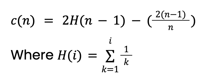
This value comes from the theory of Binary Search Trees (BST). It gives the average path length of unsuccessful searches in BST. Since Isolation Trees have an equivalent structure to BSTs, we take c(n) as the expected path length for an instance (anomaly or not). Note this value will need to be adjusted if we set a maximum depth of the tree.

Finally, we can calculate our anomaly score s(x,n):

​The score ranges between 0 and 1, and when interpreting it, we should consider three scenarios:

• If a point is an anomaly then E[h(x)] < c(n) and s → 1
• If a point is not an anomaly then E[h(x)] > c(n) and s → 0 
• If E[h(x)] = c(n) then s = 0.5

In other words, when the average path length of an instance is shorter than the expected average path length, the anomaly score will be closer to 1. However, as we will see when implementing the method, the Scikit-learn package makes further adjustments to the score. 

Isolation Forest Implementation With Python and Scikit-learn

Let’s approach the implementation step by step and start with the imports.

Imports

We have standard Python packages for data handling and visualisation (lines  2-5). We are also using the Scikit-learn implementation of Isolation Forest (line 7) and the final package is used to import our dataset (line 8).

# Imports
import pandas as pd
import numpy as np
import matplotlib.pyplot as plt
import seaborn as sns

from sklearn.ensemble import IsolationForest
from ucimlrepo import fetch_ucirepo

Dataset

We load our data directly from the UCI machine learning repository. We are using the Air Quality dataset (CC BY 4.0), which contains 9,358 instances of air quality measurements from a sensor in an Italian city. In the context of this dataset, an anomaly can be considered a sensor reading that indicates unusually high levels of pollution.

# Fetch dataset from UCI repository
air_quality = fetch_ucirepo(id=360)

Data cleaning

We do some data cleaning before applying the model. We start by selecting all features from the dataset (line 2) and then select a subset of 4 features (line 5). These are all measures of different metal oxide chemicals in the air (i.e. pollutants). We then drop any rows that have missing values (lines 8-9). In the end, we have 6,941 instances and you can see a snapshot of the feature set below.

# Convert to DataFrame
data = air_quality.data.features

# Select features
features = data[['CO(GT)', 'C6H6(GT)', 'NOx(GT)', 'NO2(GT)']]

# Drop rows with missing values (-200)
features = features.replace(-200, np.nan)
features = features.dropna()

print(features.shape)
features.head()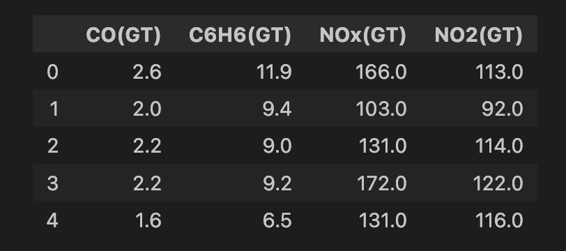

Define the training parameters

The last thing to do is define the parameters used to train the Isolation Forest. In this case, we’ll use the three values below: 

• n_estimators is the number of Isolation Trees used in the ensemble. A value of 100 is used in the Isolation Forest paper. Through experimentation, the researchers found this to produce good results over a variety of datasets. 
• contamination is the percentage of data points we expect to be anomalies. 
• sample_size is the number of instances used to train each Isolation Tree. A value of 256 is commonly used as it allows us to avoid using a maximum tree size stopping criteria. This is because we can expect reasonable maximum tree sizes of log(256) = 8.

The contamination value does not have a solid justification like the other values. It could come from previous experience. Suppose in the previous analysis we found 1% of readings to indicate high levels of pollution.  It could also come from resource constraints. For example, when analysing fraudulent transactions you may only have enough time to further analyse 5% of all transactions.  When we visualise the anomaly scores, we will see how they are adjusted using this contamination value.

# Parameters
n_estimators = 100  # Number of trees
contamination = 0.01  # Expected proportion of anomalies
sample_size = 256  # Number of samples used to train each tree

Train the Isolation Forest

Finally, we can train the Isolation Forest. If you are familiar with Sklearn, then this process should look familiar. We initialise the model using the parameters discussed above (lines 2-5). We then train the model on our feature set (line 6).

# Train Isolation Forest
iso_forest = IsolationForest(n_estimators=n_estimators,
                            contamination=contamination,
                            max_samples=sample_size,
                            random_state=42)
iso_forest.fit(features)

Calculate anomaly scores

The trained model has two useful functions: 

• decision_function will calculate the anomaly score in a similar way to what we discussed in the theory section. 
• predict will provide a binary label based on the contamination values. In our case, the 1% of instances with the worst anomaly scores will be given a value of -1. The other instances are given a value of 1.

We add the output of these functions to our dataset (lines 2-4). When we count the anomaly values (line 6) we see that 70 of the instances are labelled as anomalies.

# Calculate anomaly scores and classify anomalies
data = data.loc[features.index].copy()
data['anomaly_score'] = iso_forest.decision_function(features)
data['anomaly'] = iso_forest.predict(features)

data['anomaly'].value_counts()

We can go further and visualise all the anomaly scores. We do this using the code below:

# Visualization of the results
plt.figure(figsize=(10, 5))

# Plot normal instances
normal = data[data['anomaly'] == 1]
plt.scatter(normal.index, normal['anomaly_score'], label='Normal')

# Plot anomalies
anomalies = data[data['anomaly'] == -1]
plt.scatter(anomalies.index, anomalies['anomaly_score'], label='Anomaly')
plt.xlabel("Instance")
plt.ylabel("Anomaly Score")
plt.legend()
plt.show()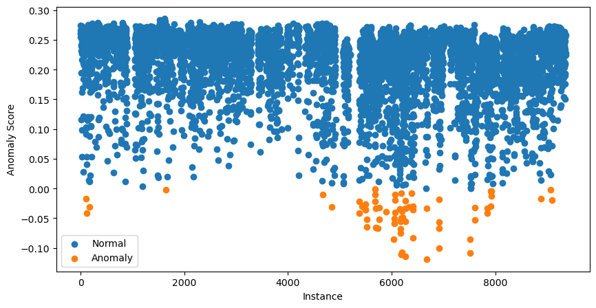

The 70 instances with the lowest anomaly scores are given in orange. These are our potential anomalies and the next step is to investigate them further.

At this point, you may be a bit confused. Didn’t we say that scores close to 1 indicate potential anomalies? 

The scores you see in the scatter plot above have been adjusted. To do this, the package first calculates an offset. This is the anomaly score percentile based on the contamination value. In our case, the offset will be the 0.99 percentile. The final scores are then given by offset - score. Doing this means that all scores below 0 suggest potential anomalies.

Further analysis

Using the scatter plot above, we can identify potential anomalies. However, this does not tell us why these have been classified as anomalies. To do that we will need to do further analysis.

For example, in the code below we create a scatter plot of all of the instances by plotting their CO(GT) value v.s. their NO2(GT) value. We also colour the points based on whether they have been classified as anomalies.

# Visualization of the results
plt.figure(figsize=(5, 5))

# Plot non-anomalies then anomalies
plt.scatter(normal['CO(GT)'], normal['NO2(GT)'], label='Normal')
plt.scatter(anomalies['CO(GT)'], anomalies['NO2(GT)'], label='Anomaly')
plt.xlabel("CO(GT)")
plt.ylabel("NO2(GT)")
plt.legend()
plt.show()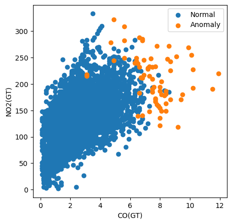

Using this plot, we can see that the CO(GT) pollutant measurement is particularly important. Notice that many of the anomalies have a value greater than 6 for this feature. However, this does not explain all of the anomalies. Some have high values for both features and others don’t seem to be anomalies due to any of the features in this plot.  This suggests that other pollutants have also contributed to the classification.

Advantages of Isolation Forest

This leads us to the main advantages of Isolation Forests over other anomaly detection methods. The first is that they can handle high-dimensional data. As we saw above, instances can be flagged as anomalies using all features, and the method can work well with far more than four features. Another key advantage is that they can find anomalies of various types.

For comparison, a simple anomaly detection method is the z-score. Using individual features, this will classify anomalies based on how far away the feature values are from their mean. However, this is only one type of anomaly. This approach also assumes features have a normal distribution and requires us to assess the z-scores for every feature in our dataset.

With Isolation Forests, we make no assumption about a feature’s distribution. The result is we can find instances that are anomalies for other reasons than being far from the mean. As we saw, we can also make classifications using all features simultaneously. This can drastically simplify our analysis, especially with large datasets.

Other considerations is that the Isolation Forest has a linear time complexity and it is unsupervised. This makes it an ideal method to detect anomalies without prior knowledge in large datasets. This is often the case in real-world applications such as fraud detection, where new types of fraud continuously emerge amongst a sea of normal transactions. 

Limitations of Isolation Forest

One notable limitation of Isolation Forest is that it may not perform as well with small datasets. This has to do with the random process in which the Isolation Trees are created. There is always a chance that normal instances have short paths or, conversely, anomalies have longer paths. With small datasets, this is more likely to happen. In other words, for Isolation Forests to work, we need enough data to average out the randomness.

Another limitation, as we have seen, is the Isolation Forest can only identify potential anomalies. It tells us nothing about why certain instances are anomalies. To do that, we need to do further analysis. Now, the advantage of identifying complex anomalies will present a challenge. Ultimately, it can take a lot of work and domain knowledge to fully explain an anomaly.

Conclusion

We explored the Isolation Forest, a powerful tool for anomaly detection across various domains. We've seen how its unique approach—isolating anomalies through random partitioning—offers advantages over traditional methods: handling high-dimensional data, identifying complex anomaly patterns, and ensuring scalability.

The practical example using Python and Scikit-learn demonstrated ease of use. 

While Isolation Forest can effectively identify potential anomalies without prior knowledge, it also has limitations, particularly when dealing with smaller datasets and its inability to explain why specific instances are considered anomalies.