Course
- Data Exploration
- Extracting the Training Data
- Building Vectorizer Classifiers
- Intermezzo: Count versus TF-IDF Features
- Conclusion

Detecting so-called “fake news” is no easy task. First, there is defining what fake news is – given it has now become a political statement. If you can find or agree upon a definition, then you must collect and properly label real and fake news (hopefully on similar topics to best show clear distinctions). Once collected, you must then find useful features to determine fake from real news.
For a more in-depth look at this problem space, I recommend taking a look at Miguel Martinez-Alvarez’s post “How can Machine Learning and AI Help Solve the Fake News Problem”.
Around the same time I read Miguel’s insightful post, I came across an open data science post about building a successful fake news detector with Bayesian models. The author even created a repository with the dataset of tagged fake and real news examples. I was curious if I could easily reproduce the results, and if I could then determine what the model had learned.
In this tutorial, you’ll walk through some of my initial exploration together and see if you can build a successful fake news detector!
Tip: if you want to learn more about Natural Language Processing (NLP) basics, consider taking the Natural Language Processing Fundamentals in Python course.
Data Exploration
To begin, you should always take a quick look at the data and get a feel for its contents. To do so, use a Pandas DataFrame and check the shape, head and apply any necessary transformations.
Extracting the Training Data
Now that the DataFrame looks closer to what you need, you want to separate the labels and set up training and test datasets.
For this notebook, I decided to focus on using the longer article text. Because I knew I would be using bag-of-words and Term Frequency–Inverse Document Frequency (TF-IDF) to extract features, this seemed like a good choice. Using longer text will hopefully allow for distinct words and features for my real and fake news data.
Building Vectorizer Classifiers
Now that you have your training and testing data, you can build your classifiers. To get a good idea if the words and tokens in the articles had a significant impact on whether the news was fake or real, you begin by using CountVectorizer and TfidfVectorizer.
You’ll see the example has a max threshhold set at .7 for the TF-IDF vectorizer tfidf_vectorizer using the max_df argument. This removes words which appear in more than 70% of the articles. Also, the built-in stop_words parameter will remove English stop words from the data before making vectors.
There are many more parameters available and you can read all about them in the scikit-learn documentation for TfidfVectorizer and CountVectorizer.
Now that you have vectors, you can then take a look at the vector features, stored in count_vectorizer and tfidf_vectorizer.
Are there any noticable issues? (Yes!)
There are clearly comments, measurements or other nonsensical words as well as multilingual articles in the dataset that you have been using. Normally, you would want to spend more time preprocessing this and removing noise, but as this tutorial just showcases a small proof of concept, you will see if the model can overcome the noise and properly classify despite these issues.
Intermezzo: Count versus TF-IDF Features
I was curious if my count and TF-IDF vectorizers had extracted different tokens. To take a look and compare features, you can extract the vector information back into a DataFrame to use easy Python comparisons.
As you can see by running the cells below, both vectorizers extracted the same tokens, but obviously have different weights. Likely, changing the max_df and min_df of the TF-IDF vectorizer could alter the result and lead to different features in each.
count_df = pd.DataFrame(count_train.A, columns=count_vectorizer.get_feature_names())tfidf_df = pd.DataFrame(tfidf_train.A, columns=tfidf_vectorizer.get_feature_names())difference = set(count_df.columns) - set(tfidf_df.columns)differenceset()
print(count_df.equals(tfidf_df))Falsecount_df.head()| 00 | 000 | 0000 | 00000031 | 000035 | 00006 | 0001 | 0001pt | 000ft | 000km | ... | حلب | عربي | عن | لم | ما | محاولات | من | هذا | والمرضى | ยงade | |
|---|---|---|---|---|---|---|---|---|---|---|---|---|---|---|---|---|---|---|---|---|---|
| 0 | 0 | 0 | 0 | 0 | 0 | 0 | 0 | 0 | 0 | 0 | ... | 0 | 0 | 0 | 0 | 0 | 0 | 0 | 0 | 0 | 0 |
| 1 | 0 | 0 | 0 | 0 | 0 | 0 | 0 | 0 | 0 | 0 | ... | 0 | 0 | 0 | 0 | 0 | 0 | 0 | 0 | 0 | 0 |
| 2 | 0 | 0 | 0 | 0 | 0 | 0 | 0 | 0 | 0 | 0 | ... | 0 | 0 | 0 | 0 | 0 | 0 | 0 | 0 | 0 | 0 |
| 3 | 0 | 0 | 0 | 0 | 0 | 0 | 0 | 0 | 0 | 0 | ... | 0 | 0 | 0 | 0 | 0 | 0 | 0 | 0 | 0 | 0 |
| 4 | 0 | 0 | 0 | 0 | 0 | 0 | 0 | 0 | 0 | 0 | ... | 0 | 0 | 0 | 0 | 0 | 0 | 0 | 0 | 0 | 0 |
5 rows × 56922 columns
tfidf_df.head()| 00 | 000 | 0000 | 00000031 | 000035 | 00006 | 0001 | 0001pt | 000ft | 000km | ... | حلب | عربي | عن | لم | ما | محاولات | من | هذا | والمرضى | ยงade | |
|---|---|---|---|---|---|---|---|---|---|---|---|---|---|---|---|---|---|---|---|---|---|
| 0 | 0.0 | 0.0 | 0.0 | 0.0 | 0.0 | 0.0 | 0.0 | 0.0 | 0.0 | 0.0 | ... | 0.0 | 0.0 | 0.0 | 0.0 | 0.0 | 0.0 | 0.0 | 0.0 | 0.0 | 0.0 |
| 1 | 0.0 | 0.0 | 0.0 | 0.0 | 0.0 | 0.0 | 0.0 | 0.0 | 0.0 | 0.0 | ... | 0.0 | 0.0 | 0.0 | 0.0 | 0.0 | 0.0 | 0.0 | 0.0 | 0.0 | 0.0 |
| 2 | 0.0 | 0.0 | 0.0 | 0.0 | 0.0 | 0.0 | 0.0 | 0.0 | 0.0 | 0.0 | ... | 0.0 | 0.0 | 0.0 | 0.0 | 0.0 | 0.0 | 0.0 | 0.0 | 0.0 | 0.0 |
| 3 | 0.0 | 0.0 | 0.0 | 0.0 | 0.0 | 0.0 | 0.0 | 0.0 | 0.0 | 0.0 | ... | 0.0 | 0.0 | 0.0 | 0.0 | 0.0 | 0.0 | 0.0 | 0.0 | 0.0 | 0.0 |
| 4 | 0.0 | 0.0 | 0.0 | 0.0 | 0.0 | 0.0 | 0.0 | 0.0 | 0.0 | 0.0 | ... | 0.0 | 0.0 | 0.0 | 0.0 | 0.0 | 0.0 | 0.0 | 0.0 | 0.0 | 0.0 |
5 rows × 56922 columns
Comparing Models
Now it's time to train and test your models.
Here, you'll begin with an NLP favorite, MultinomialNB. You can use this to compare TF-IDF versus bag-of-words. My intuition was that bag-of-words (aka CountVectorizer) would perform better with this model. (For more reading on multinomial distribution and why it works best with integers, check out this fairly succinct explanation from a UPenn statistics course).
I personally find Confusion Matrices easier to compare and read, so I used the scikit-learn documentation to build some easily-readable confusion matrices (thanks open source!). A confusion matrix shows the proper labels on the main diagonal (top left to bottom right). The other cells show the incorrect labels, often referred to as false positives or false negatives. Depending on your problem, one of these might be more significant. For example, for the fake news problem, is it more important that we don't label real news articles as fake news? If so, we might want to eventually weight our accuracy score to better reflect this concern.
Other than Confusion Matrices, scikit-learn comes with many ways to visualize and compare your models. One popular way is to use a ROC Curve. There are many other ways to evaluate your model available in the scikit-learn metrics module.
def plot_confusion_matrix(cm, classes, normalize=False, title='Confusion matrix', cmap=plt.cm.Blues): """ See full source and example: http://scikit-learn.org/stable/auto_examples/model_selection/plot_confusion_matrix.html This function prints and plots the confusion matrix. Normalization can be applied by setting `normalize=True`. """ plt.imshow(cm, interpolation='nearest', cmap=cmap) plt.title(title) plt.colorbar() tick_marks = np.arange(len(classes)) plt.xticks(tick_marks, classes, rotation=45) plt.yticks(tick_marks, classes) if normalize: cm = cm.astype('float') / cm.sum(axis=1)[:, np.newaxis] print("Normalized confusion matrix") else: print('Confusion matrix, without normalization') thresh = cm.max() / 2. for i, j in itertools.product(range(cm.shape[0]), range(cm.shape[1])): plt.text(j, i, cm[i, j], horizontalalignment="center", color="white" if cm[i, j] > thresh else "black") plt.tight_layout() plt.ylabel('True label') plt.xlabel('Predicted label')clf = MultinomialNB() clf.fit(tfidf_train, y_train)pred = clf.predict(tfidf_test)score = metrics.accuracy_score(y_test, pred)print("accuracy: %0.3f" % score)cm = metrics.confusion_matrix(y_test, pred, labels=['FAKE', 'REAL'])plot_confusion_matrix(cm, classes=['FAKE', 'REAL'])accuracy: 0.857Confusion matrix, without normalization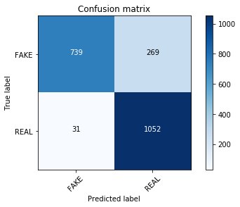
clf = MultinomialNB() clf.fit(count_train, y_train)pred = clf.predict(count_test)score = metrics.accuracy_score(y_test, pred)print("accuracy: %0.3f" % score)cm = metrics.confusion_matrix(y_test, pred, labels=['FAKE', 'REAL'])plot_confusion_matrix(cm, classes=['FAKE', 'REAL'])accuracy: 0.893Confusion matrix, without normalization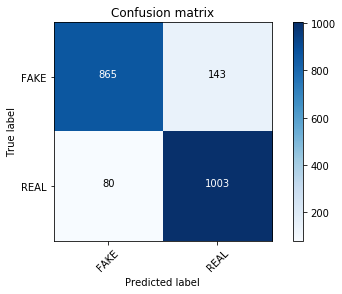
And indeed, with absolutely no parameter tuning, your count vectorized training set count_train is visibly outperforming your TF-IDF vectors!
Testing Linear Models
There are a lot of great write-ups about how linear models work well with TF-IDF vectorizers (take a look at word2vec for classification, SVM reference in scikit-learn text analysis, and many more).
So you should use a SVM, right?
Well, I recently watched Victor Lavrenko's lecture on text classification and he compares Passive Aggressive classifiers to linear SVMs for text classification. We'll test this approach (which has some significant speed benefits and permanent learning disadvantages) with the fake news dataset.
linear_clf = PassiveAggressiveClassifier(n_iter=50) linear_clf.fit(tfidf_train, y_train)pred = linear_clf.predict(tfidf_test)score = metrics.accuracy_score(y_test, pred)print("accuracy: %0.3f" % score)cm = metrics.confusion_matrix(y_test, pred, labels=['FAKE', 'REAL'])plot_confusion_matrix(cm, classes=['FAKE', 'REAL'])accuracy: 0.936Confusion matrix, without normalization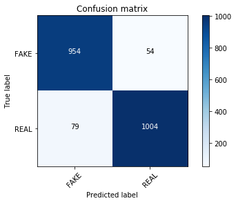
Wow!
I'm impressed. The confusion matrix looks different and the model classifies our fake news a bit better. We can test if tuning the alpha value for a MultinomialNB creates comparable results. You can also use parameter tuning with grid search for a more exhaustive search.
clf = MultinomialNB(alpha=0.1) last_score = 0for alpha in np.arange(0,1,.1): nb_classifier = MultinomialNB(alpha=alpha) nb_classifier.fit(tfidf_train, y_train) pred = nb_classifier.predict(tfidf_test) score = metrics.accuracy_score(y_test, pred) if score > last_score: clf = nb_classifier print("Alpha: {:.2f} Score: {:.5f}".format(alpha, score))Alpha: 0.00 Score: 0.61502Alpha: 0.10 Score: 0.89766Alpha: 0.20 Score: 0.89383Alpha: 0.30 Score: 0.89000Alpha: 0.40 Score: 0.88570Alpha: 0.50 Score: 0.88427Alpha: 0.60 Score: 0.87470Alpha: 0.70 Score: 0.87040Alpha: 0.80 Score: 0.86609Alpha: 0.90 Score: 0.85892Not quite... At this point, it might be interesting to perform parameter tuning across all of the classifiers, or take a look at some other scikit-learn Bayesian classifiers. You could also test with a Support Vector Machine (SVM) to see if that outperforms the Passive Aggressive classifier.
But I am a bit more curious about what the Passive Aggressive model actually has learned. So let's move onto introspection.
Introspecting models
So fake news is solved, right? We achieved 93% accuracy on my dataset so let's all close up shop and go home.
Not quite, of course. I am wary at best of these results given how much noise we saw in the features. There is a great write-up on StackOverflow with this incredibly useful function for finding vectors that most affect labels. It only works for binary classificaiton (classifiers with 2 classes), but that's good news for you, since you only have FAKE or REAL labels.
Using your best performing classifier with your TF-IDF vector dataset (tfidf_vectorizer) and Passive Aggressive classifier (linear_clf), inspect the top 30 vectors for fake and real news:
FAKE -4.86382369883 2016FAKE -4.13847157932 hillaryFAKE -3.98994974843 octoberFAKE -3.10552662226 shareFAKE -2.99713810694 novemberFAKE -2.9150746075 articleFAKE -2.54532100449 printFAKE -2.47115243995 advertisementFAKE -2.35915304509 sourceFAKE -2.31585837413 emailFAKE -2.27985826579 electionFAKE -2.2736680857 octFAKE -2.25253568246 warFAKE -2.19663276969 mosulFAKE -2.17921304122 podestaFAKE -1.99361009573 novFAKE -1.98662624907 comFAKE -1.9452527887 establishmentFAKE -1.86869495684 corporateFAKE -1.84166664376 wikileaksFAKE -1.7936566878 26FAKE -1.75686475396 donaldFAKE -1.74951154055 snipFAKE -1.73298170472 mainstreamFAKE -1.71365596627 ukFAKE -1.70917804969 ayotteFAKE -1.70781651904 entireFAKE -1.68272667818 jewishFAKE -1.65334397724 youtubeFAKE -1.6241703128 pipelineREAL 4.78064061698 saidREAL 2.68703967567 tuesdayREAL 2.48309800829 gopREAL 2.45710670245 islamicREAL 2.44326123901 saysREAL 2.29424417889 cruzREAL 2.29144842597 marriageREAL 2.20500735471 candidatesREAL 2.19136552672 conservativeREAL 2.18030834903 mondayREAL 2.05688105375 attacksREAL 2.03476457362 rushREAL 1.9954523319 continueREAL 1.97002430576 fridayREAL 1.95034103105 conventionREAL 1.94620720989 senREAL 1.91185661202 jobsREAL 1.87501303774 debateREAL 1.84059602241 presumptiveREAL 1.80111133252 sayREAL 1.80027216061 sundayREAL 1.79650823765 marchREAL 1.79229792108 parisREAL 1.74587899553 securityREAL 1.69585506276 conservativesREAL 1.68860503431 recountsREAL 1.67424302821 dealREAL 1.67343398121 campaignREAL 1.66148582079 foxREAL 1.61425630518 attackYou can also do this in a pretty obvious way with only a few lines of Python, by zipping your coefficients to your features and taking a look at the top and bottom of your list.
feature_names = tfidf_vectorizer.get_feature_names()### Most realsorted(zip(clf.coef_[0], feature_names), reverse=True)[:20][(-6.2573612147015822, 'trump'), (-6.4944530943126777, 'said'), (-6.6539784739838845, 'clinton'), (-7.0379446628670728, 'obama'), (-7.1465399833812278, 'sanders'), (-7.2153760086475112, 'president'), (-7.2665628057416169, 'campaign'), (-7.2875931446681514, 'republican'), (-7.3411184585990643, 'state'), (-7.3413571102479054, 'cruz'), (-7.3783124419854254, 'party'), (-7.4468806724578904, 'new'), (-7.4762888011545883, 'people'), (-7.547225599514773, 'percent'), (-7.5553074094582335, 'bush'), (-7.5801506339098932, 'republicans'), (-7.5855405012652435, 'house'), (-7.6344781725203141, 'voters'), (-7.6484824436952987, 'rubio'), (-7.6734836186463795, 'states')]### Most fakesorted(zip(clf.coef_[0], feature_names))[:20][(-11.349866225220305, '0000'), (-11.349866225220305, '000035'), (-11.349866225220305, '0001'), (-11.349866225220305, '0001pt'), (-11.349866225220305, '000km'), (-11.349866225220305, '0011'), (-11.349866225220305, '006s'), (-11.349866225220305, '007'), (-11.349866225220305, '007s'), (-11.349866225220305, '008s'), (-11.349866225220305, '0099'), (-11.349866225220305, '00am'), (-11.349866225220305, '00p'), (-11.349866225220305, '00pm'), (-11.349866225220305, '014'), (-11.349866225220305, '015'), (-11.349866225220305, '018'), (-11.349866225220305, '01am'), (-11.349866225220305, '020'), (-11.349866225220305, '023')]So, clearly there are certain words which might show political intent and source in the top fake features (such as the words corporate and establishment).
Also, the real news data uses forms of the verb "to say" more often, likely because in newspapers and most journalistic publications sources are quoted directly ("German Chancellor Angela Merkel said...").
To extract the full list from your current classifier and take a look at each token (or easily compare tokens from classifier to classifier), you can easily export it like so.
tokens_with_weights = sorted(list(zip(feature_names, clf.coef_[0])))Intermezzo: HashingVectorizer
Another vectorizer used sometimes for text classification is a HashingVectorizer. HashingVectorizers require less memory and are faster (because they are sparse and use hashes rather than tokens) but are more difficult to introspect. You can read a bit more about the pros and cons of using HashingVectorizer in the scikit-learn documentation if you are interested.
You can give it a try and compare its results versus the other vectorizers. It performs fairly well, with better results than the TF-IDF vectorizer using MultinomialNB (this is somewhat expected due to the same reasons CountVectorizers perform better), but not as well as the TF-IDF vectorizer with Passive Aggressive linear algorithm.
hash_vectorizer = HashingVectorizer(stop_words='english', non_negative=True)hash_train = hash_vectorizer.fit_transform(X_train)hash_test = hash_vectorizer.transform(X_test)clf = MultinomialNB(alpha=.01)clf.fit(hash_train, y_train)pred = clf.predict(hash_test)score = metrics.accuracy_score(y_test, pred)print("accuracy: %0.3f" % score)cm = metrics.confusion_matrix(y_test, pred, labels=['FAKE', 'REAL'])plot_confusion_matrix(cm, classes=['FAKE', 'REAL'])accuracy: 0.902Confusion matrix, without normalization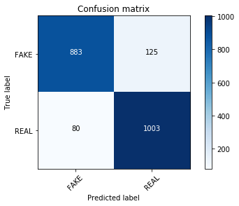
clf = PassiveAggressiveClassifier(n_iter=50)clf.fit(hash_train, y_train)pred = clf.predict(hash_test)score = metrics.accuracy_score(y_test, pred)print("accuracy: %0.3f" % score)cm = metrics.confusion_matrix(y_test, pred, labels=['FAKE', 'REAL'])plot_confusion_matrix(cm, classes=['FAKE', 'REAL'])accuracy: 0.921Confusion matrix, without normalization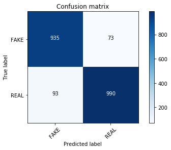
Conclusion
So was your fake news classifier experiment a success? Definitely not.
But you did get to play around with a new dataset, test out some NLP classification models and introspect how successful they were? Yes.
As expected from the outset, defining fake news with simple bag-of-words or TF-IDF vectors is an oversimplified approach. Especially with a multilingual dataset full of noisy tokens. If you hadn't taken a look at what your model had actually learned, you might have thought the model learned something meaningful. So, remember: always introspect your models (as best you can!).
I would be curious if you find other trends in the data I might have missed. I will be following up with a post on how different classifiers compare in terms of important features on my blog. If you spend some time researching and find anything interesting, feel free to share your findings and notes in the comments or you can always reach out on Twitter (I'm @kjam).
I hope you had some fun exploring a new NLP dataset with me!
Take a look at DataCamp's Python Machine Learning: Scikit-Learn Tutorial.
