DeepSeek mHC Explained: Scaling LLMs Beyond FLOPs

DeepSeek’s mHC (Manifold-Constrained Hyper-Connections) addresses a problem most teams face when scaling LLMs: you can keep adding GPUs, but at some point, training becomes unstable and throughput stops improving.

Here’s the core idea:

• At scale, the real limits are often memory bandwidth, GPU-to-GPU communication, and latency overhead.
• Hyper-Connections (HC) try to improve model capacity by letting information flow through richer residual paths without increasing per-layer FLOPs too much. But that extra mixing can break the “identity shortcut” that made residual networks stable in the first place, causing training to blow up.
• mHC fixes this by constraining how those residual paths mix. The residual mixing is forced to behave like a well-behaved weighted average (a doubly stochastic matrix, enforced using Sinkhorn–Knopp), which keeps signals and gradients from exploding or dying out.

Hyper-Connections improve connectivity and capacity, but Manifold-Constrained Hyper-Connections(mHCs) make that upgrade stable and scalable, without ignoring the real bottlenecks like memory bandwidth and communication.

If you’re keen to learn more about some of the principles covered in this tutorial, I recommend checking out the Transformer Models with PyTorch course and the Deep Learning with PyTorch course.

What is mHC? From Residual Connections to Hyper-Connections

In this section, I’ll unpack the need to move beyond plain residual connections, how HC tried to solve that, and why mHC is the fix that makes the idea work at LLM scale.

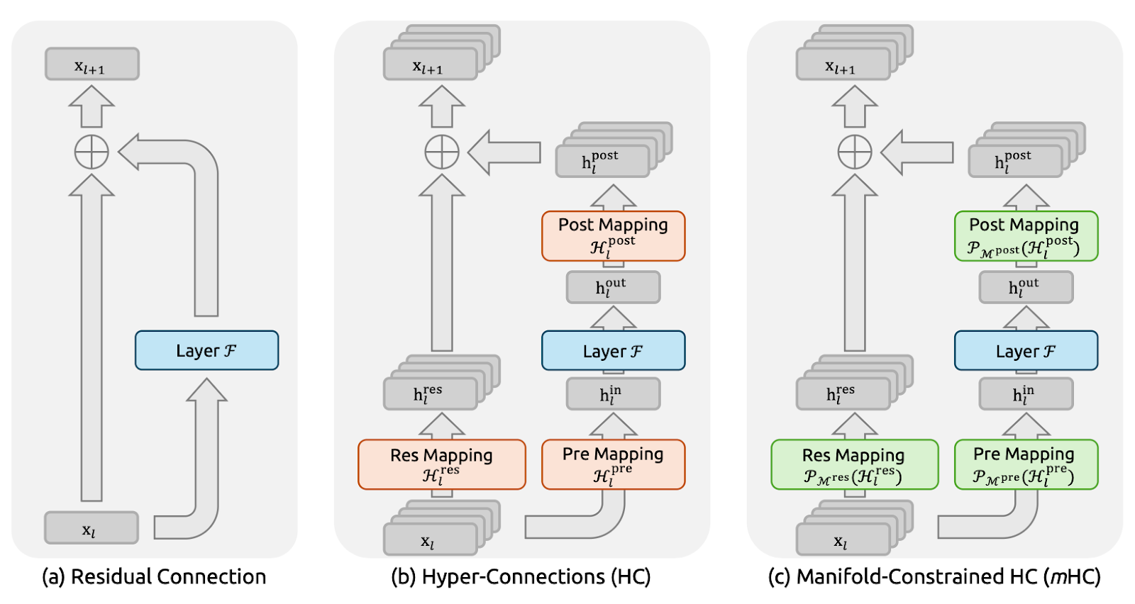
Figure 1: Illustrations of Residual Connection Paradigms (mHC paper)

Residual connections (Figure a) provide each layer with an identity shortcut, allowing signals and gradients to flow cleanly through very deep networks. 

DeepSeek explicitly used this identity mapping principle as the starting point for the mHC paper. The downside is that a plain residual path is also too restrictive, so it doesn’t allow much information exchange inside the residual stream. 

While Hyper-Connections (HC) (Figure b) were the natural next step, which instead of one residual stream, expands into n parallel streams and adds learnable pre/post/residual mappings so streams can mix and share information. This increases expressivity without necessarily exploding per-layer FLOPs. 

But at a large scale, HC runs into two big issues. First, because the streams mix freely at every layer, those small mixings pile up as you go deeper. Over many layers, the network can stop behaving like a clean “skip connection,” and signals or gradients can blow up or fade out, making the training unstable. Second, even if the extra computations are simple, the hardware cost rises fast.

Manifold-Constrained Hyper-Connections (mHC) (Figure c) keeps the extra connectivity of HC, but makes it safe to train like a ResNet. 

The main idea is that instead of letting the residual streams mix in any way, mHC forces the mixing to follow strict rules. In the paper, it does this by turning the mixing matrix into a well-behaved “weighted average”, using a procedure called Sinkhorn–Knopp. The result is that even after many layers, the mixing stays stable, and signals and gradients do not explode or vanish.

In short, we moved from residual connections to mHC because we wanted richer information flow rather than a single skip path.

mHC Key Concepts

At a high level, mHC keeps Hyper-Connection’s multi-stream mixing, but puts hard guardrails on the mixing so it behaves like a stable, ResNet-style skip path even when we stack hundreds of layers. 

The authors constrain the residual mixing matrix Hlres​ so it stays well-behaved across depth, while still allowing streams to exchange information.

Concretely, mHC forces Hlres​​ to be doubly stochastic, i.e., all entries are non-negative, and each row and each column sums to 1. That makes the residual stream act like a controlled weighted average. 

This highlights that the mapping is non-expansive (spectral norm bounded by 1), stays stable when multiplied across layers (closure under multiplication), and has an intuitive mixing as averaging/permutation blending interpretation via the Birkhoff polytope. It also constrains the pre/post mappings to be non-negative to avoid signal cancellation. 

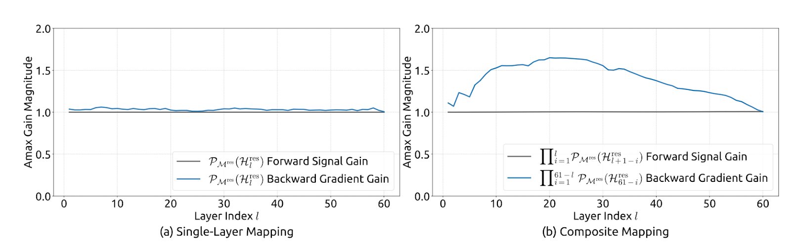
Figure 2: Propagation Stability of Manifold-Constrained Hyper-Connections(mHC paper)

Implementation-wise, the paper keeps it practical by computing unconstrained raw mappings Hlpre, Hlpost, and  Hlres from the current layer’s multi-stream state (they flatten xl to preserve full context), then project them into the constrained forms. Hlpre and Hlpost​​ are obtained with a sigmoid-based constraint, while ​Hlres is projected using Sinkhorn–Knopp exponentiate to make entries positive, then alternate row/column normalizations until sums are 1.

The authors also report implementing mHC (with n=4) at scale with only ~6.7% training-time overhead, mainly by aggressively reducing memory traffic. They reordered the parts of RMSNorm for efficiency, used kernel fusion (including implementing Sinkhorn iterations inside a single kernel with a custom backward), fused the application of  Hlpost​​ and Hlres with residual merge to cut reads/writes, used selective recomputing to avoid storing large intermediate activations, and overlapping communication in an extended DualPipe schedule to hide pipeline-stage latency.

Optimizing mHC: Systems Techniques 

Stability alone isn’t enough. If mHC adds too much memory traffic or GPU-to-GPU communication, we lose on throughput. So the authors paired the mHC method with a set of infrastructure optimizations designed to stay friendly to the memory wall.

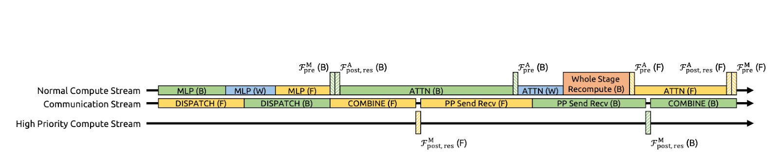
Figure 3: Communication-Computation Overlapping for mHC(mHC paper)

Kernel fusion to cut memory reads/writes

The authors speed up mHC by fusing several steps into one GPU kernel. Instead of applying Hlpost​, Hlres, and then merging back into the residual stream as separate passes (which forces the GPU to write intermediate tensors to memory and read them back), they do these operations in a single pass. 

This cuts memory traffic substantially. The kernel now reads about (n+1)C values instead of (3n+1)C and writes about nC values instead of 3nC. Here, C is the hidden size (features per stream) and n is the number of residual streams, so nC is the size of the widened residual state. Fewer reads/writes means less data moving to and from memory. 

The paper also suggests implementing most kernels using TileLang to utilize memory bandwidth in a better way. 

Recomputation to control activation memory

Multi-stream mHC increases the amount of intermediate activations you’d normally have to store for backprop, which can blow up GPU memory and force smaller batches or more aggressive checkpointing. 

To avoid that, the paper suggests a simple trick: don’t store the mHC intermediates after the forward pass. Instead, recompute the lightweight mHC kernels during the backward pass, while skipping recomputation of the expensive Transformer layer F. 

This reduces memory pressure and helps maintain higher effective throughput. A practical constraint is that these recomputation blocks should line up with pipeline stage boundaries; otherwise, pipeline scheduling becomes messy.

Communication-aware scheduling with DualPipe overlap

At scale, pipeline parallelism is common, but mHC’s n-stream design increases the amount of data that must cross stage boundaries, which can add noticeable communication stalls. 

DeepSeek optimizes this by extending DualPipe so that communication and computation overlap at pipeline boundaries. This means that the GPUs do useful work while transfers take place instead of sitting idle waiting for sends/receives to finish. They also run some kernels on a high-priority compute stream, so compute doesn’t block communication progress. The result is that the extra communication cost from mHC is partially hidden, improving end-to-end training efficiency

Hot Spots 

Even if we don’t implement mHC, DeepSeek’s framing is a good way to spot where the system is actually losing time.

• Long-context workloads: Long prompts make prefill expensive because attention has to move a lot of data through memory. During decode, the KV cache keeps growing, which increases memory reads per token. Together, these push memory bandwidth limits and often cause fragmentation or inefficient batching.
• MoE routing and expert parallelism: With Mixture of Experts (MoE), the cost isn’t just about compute. It’s the routing, token exchange, and cross-GPU communication needed to send tokens to experts and gather outputs. DeepSeek’s DualPipe overlap focuses on hiding the pipeline communication behind computation, which MoE needs at scale.
• Multi-tenant and small-batch traffic: In real deployments, requests don’t arrive in neat large batches. We get smaller, inconsistent batches, mixed sequence lengths, and weaker cache reuse. That hurts batching efficiency and inflates tail latency, so the memory bandwidth and scheduling become the bottleneck.

KV Cache and Memory Traffic

Even though mHC is mainly a training idea, the paper’s core lesson applies directly to inference. The paper focuses on optimizing not only for FLOPs, but also for memory traffic, communication, and latency. The biggest proof is long-context decoding, where the rough KV-cache estimate is:

KV_bytes ≈  2 x L x T x H x bytes_per_elem x batch

For FP16/BF16, the bytes_per_elem value is 2. For example, with a typical shape ( L=32, H=4096, batch=1), 8K tokens is ~4 GB of KV, while 128K tokens is ~64 GB, so even if compute stays reasonable, the memory could still explode, and you become bandwidth-bound. 

That’s why practical inference optimizations focus on reducing memory movement using techniques like KV cache quantization, paged KV and eviction, efficient attention kernels (FlashAttention-family), continuous batching and shape bucketing, and communication-aware parallelism. 

The goal is to keep the performance gains without paying a hidden tax in memory reads/writes and synchronization.

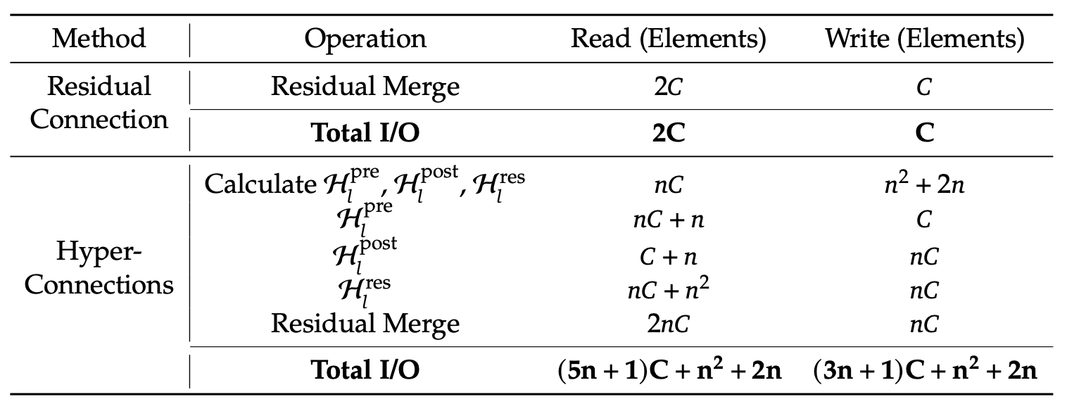
Table 1: Comparison of Memory Access Costs Per Token(mHC paper)

DeepSeek reports mHC consistently outperforming the baseline and surpassing HC on most benchmarks for 27B models, including +2.1% on BBH and +2.3% on DROP compared to HC. This shows that mHC translates into better results at scale.

Conclusion

The key takeaway from this paper is that scaling LLMs isn’t just a FLOPs problem; it’s equally a stability and systems problem. Hyper-Connections (HC) enhance model capacity by expanding the residual stream and allowing multiple streams to mix, but at large depths, this mixing compounds into a composite mapping that can deviate significantly from an identity path, leading to signal/gradient explosion or vanishing, and training blow-ups.

mHC fixes this by putting guardrails on that mixing by constraining the residual mixing matrix to be doubly stochastic (non-negative, rows/columns sum to 1), enforced via Sinkhorn–Knopp, so the residual path behaves like a controlled weighted average and remains stable even when you stack many layers.

DeepSeek also treats runtime efficiency as part of the method. They used kernel fusion to reduce high-bandwidth memory reads/writes, and selective recomputation to minimize activation memory. 

Additionally, they extended DualPipe to overlap communication with computation, ensuring that pipeline stalls don’t erase the gains. The result is not only more stable training, but also better downstream performance at scale.

If you’re keen to learn more about LLM application development, I recommend checking out the Developing LLM Applications with LangChain course.