Taylor-reeksen: van benaderingen tot optimalisatie

Heb je je ooit afgevraagd hoe een computer eigenlijk een functie als sin(x) of eˣ berekent?

Computers kunnen de meeste wiskundige functies niet rechtstreeks evalueren. Ze kunnen alleen optellen, aftrekken, vermenigvuldigen en delen. Dus wanneer je in Python math.sin(0.5) aanroept, moet dat worden omgezet in een reeks basisbewerkingen. Dat gebeurt met polynomiale benaderingen, en Taylor-reeksen vormen daar de wiskundige basis van.

Een Taylor-reeks laat je bijna elke vloeiende functie herschrijven als een oneindige som van eenvoudigere termen, elk opgebouwd uit de afgeleiden van de functie in één punt. Als je dit idee snapt, vallen veel dingen in data science en machine learning op hun plek - van hoe gradient descent werkt tot waarom bepaalde activatiefuncties zich gedragen zoals ze doen.

In dit artikel neem ik je mee door wat Taylor-reeksen zijn, hoe ze wiskundig werken, waar je ze tegenkomt in data science en machine learning, en hoe ze zich verhouden tot andere soorten reeksen die je zult zien.

Taylor-reeksen definiëren

Taylor-reeksen bestaan al eeuwen. Brook Taylor introduceerde ze in 1715, al leverden James Gregory en Colin Maclaurin ook belangrijke bijdragen aan het idee.

Het doel was om complexe functies weer te geven met polynomen, die veel makkelijker te hanteren zijn.

Een Taylor-reeks benadert een functie door die uit te drukken als een oneindige som van termen, elk afgeleid van de afgeleiden van de functie in één punt. Hoe meer termen je opneemt, hoe dichter de benadering bij de echte functie komt.

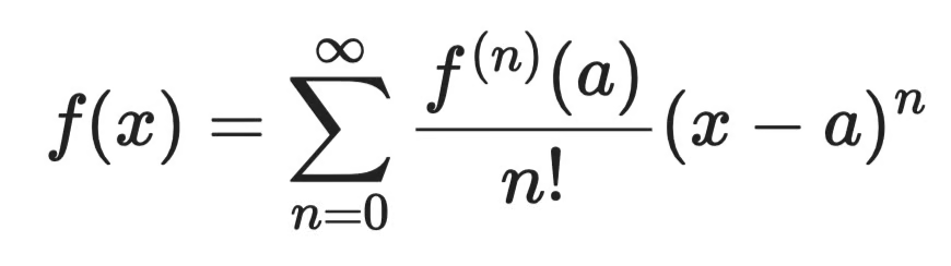
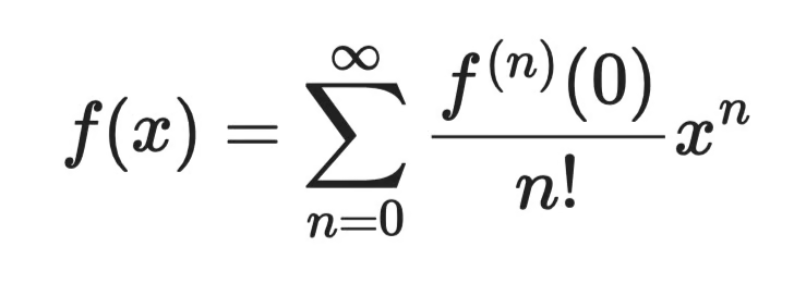
De algemene formule is als volgt:

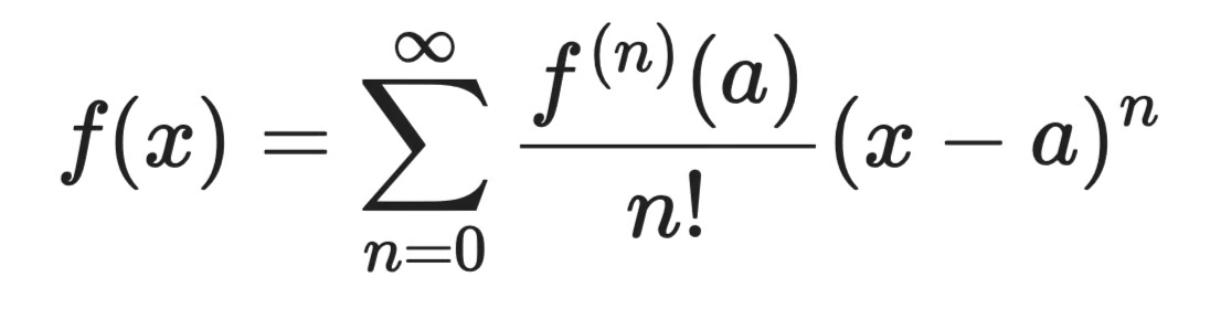
Algemene Taylorreeks-formule

Elke term in deze som bestaat uit drie componenten:

• f⁽ⁿ⁾(a) - de n-de afgeleide van de functie geëvalueerd in het centrumpunt a

• n! - de faculteit van n, die voorkomt dat de termen ongebreideld groeien

• (x - a)ⁿ - de expandeterm, die meet hoe ver x van het centrumpunt af ligt

Het centrumpunt a is waar je de reeks aan verankert. Als a = 0, krijg je een speciaal geval dat een Maclaurin-reeks heet - daarover later meer.

Een concreet voorbeeld: eˣ

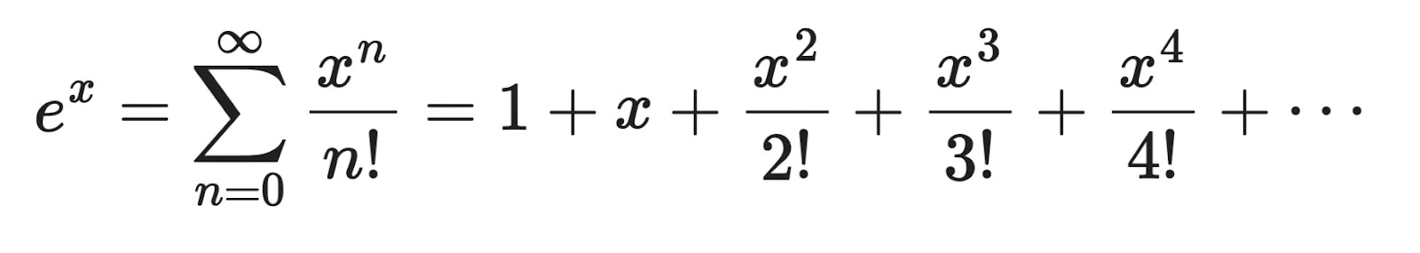
De exponentiële functie eˣ is een perfect eerste voorbeeld. De afgeleide is zichzelf, dus f⁽ⁿ⁾(0) = 1 voor elke n. Gecentreerd op a = 0 wordt de Taylor-reeks:

Concreet voorbeeld

Stel, je wilt e⁰·⁵ benaderen. Vul gewoon x = 0.5 in de eerste vier termen in - hier is een Python-voorbeeld:

x = 0.5
approx = 1 + x + x**2/2 + x**3/6
print(approx)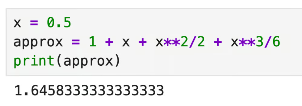

Concreet voorbeeld in Python

De werkelijke waarde van e⁰·⁵ is ongeveer 1.6487. Met slechts vier termen zit je al binnen 0,2% van het juiste antwoord. Voeg meer termen toe, en de benadering wordt nog strakker.

Dat is de kracht van Taylor-reeksen.

Functies als eˣ, sin(x) en cos(x) zijn lastig direct te evalueren, maar hun Taylor-reeksen herleiden ze tot basisrekenwerk. Precies waar een computer mee overweg kan.

Wiskundige eigenschappen van Taylor-reeksen

Een Taylor-reeks is alleen nuttig als hij daadwerkelijk convergeert naar de functie die je probeert te benaderen. Laten we bekijken wat dat betekent en wat er gebeurt als dat niet zo is.

Taylorreeks-expansie

Als je een Taylor-reeks uitbreidt, bouw je stap voor stap een veelterm op. Elke term voegt meer informatie toe over het gedrag van de functie in de buurt van het centrumpunt a.

Neem sin(x) gecentreerd op a = 0:

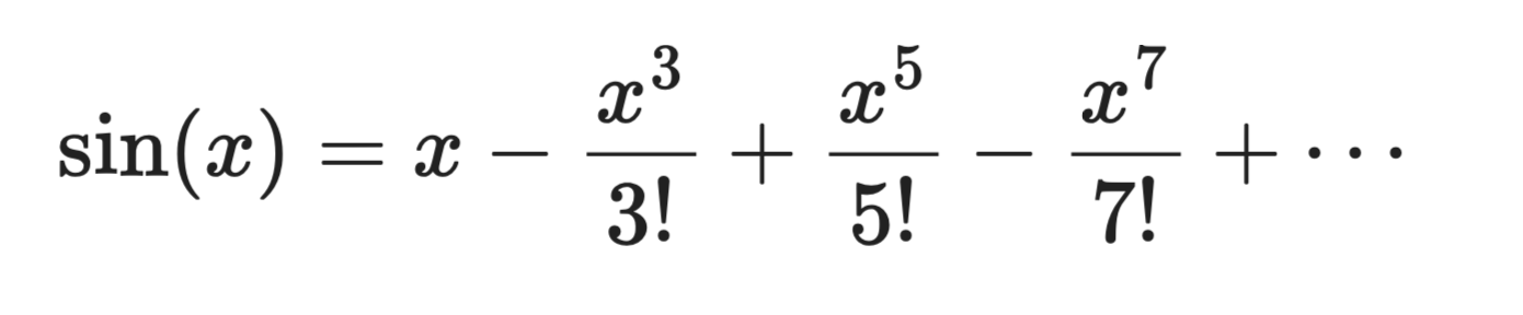
Taylorreeks-expansie

De eerste term, x, is een ruwe lineaire benadering. Voeg de tweede term toe en de kromme komt dichterbij. Voeg meer termen toe, en het polynoom begint er precies uit te zien als sin(x) in de buurt van x = 0.

Kort gezegd: met een expansie ruil je een exacte maar lastig te berekenen functie in voor een polynoom waar je daadwerkelijk mee kunt werken.

Taylorreeks-benadering

Je zult nooit oneindig veel termen uitrekenen. In de praktijk stop je na een paar termen en accepteer je een kleine fout. Het resultaat heet een afgeknotte Taylor-reeks, en de fout die dat introduceert heet de afsnijfout.

De restterm van Lagrange geeft je een bovengrens voor die fout. Voor een reeks die na n termen wordt afgebroken:

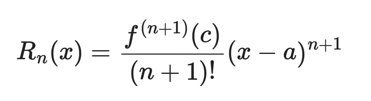
Lagrange-restterm

Waarbij c een punt is tussen x en a. Je kent c niet exact, maar je kunt f⁽ⁿ⁺¹⁾(c) begrenzen als je weet hoe groot de afgeleiden van je functie kunnen worden.

Zo kun je het interpreteren

• Hoe verder x van het centrumpunt a ligt, hoe groter de fout

• Hoe meer termen je opneemt, hoe kleiner de fout

• Functies met grote, snelgroeiende afgeleiden zijn lastiger nauwkeurig te benaderen

Stel dat je sin(0.1) benadert met drie termen:

x = 0.1
approx = x - x**3/6 + x**5/120
print(approx)       
print(np.sin(0.1))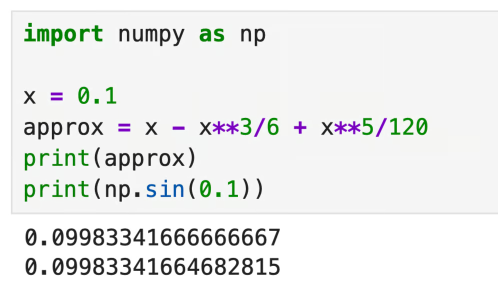  

Benadering in Python

Drie termen leveren je nauwkeurigheid tot op tien decimalen wanneer x dicht bij 0 ligt. Dat is afsnijfout in actie - klein, maar niet nul.

Convergentie van Taylor-reeksen

Een Taylor-reeks convergeert in een punt x als de partieelsommen steeds dichter bij een vaste waarde komen naarmate je meer termen toevoegt. Die vaste waarde zou f(x) moeten zijn - maar dat is niet altijd gegarandeerd.

De convergentiestraal R vertelt je hoe ver vanaf het centrumpunt de reeks geldig blijft. Binnen die straal convergeert de reeks. Daarbuiten groeien de termen in plaats van te krimpen, en valt de benadering uiteen.

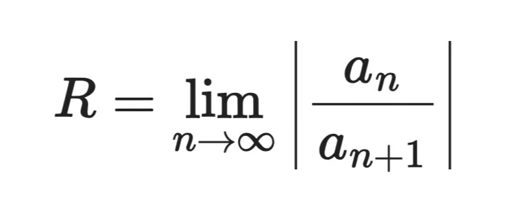
Convergentieformule

Verschillende functies hebben verschillende stralen:

• eˣ, sin(x) en cos(x) convergeren voor alle waarden van x, dus R = ∞

• ln(1 + x) convergeert alleen voor -1 < x <= 1, dus R = 1

• 1/1-x convergeert voor |x| < 1, dus R = 1

Een functie kan ook een oneindige convergentiestraal hebben maar toch niet gelijk zijn aan haar Taylor-reeks op bepaalde punten. Dat heet niet-analytisch, en het is een randgeval om te kennen, ook al kom je het zelden tegen in data science.

Controleer dus altijd of x binnen de convergentiestraal valt voordat je een Taylor-benadering vertrouwt.

Taylor-reeksen in data science en machine learning

Taylor-reeksen duiken op meer plekken op dan je zou verwachten - van fysicasimulaties tot het oplossen van differentiaalvergelijkingen. Maar hun grootste impact in je dagelijkse werk als data scientist zit in optimalisatie en modelbenadering.

Optimalisatie en gradient descent

Elke keer dat je een machinelearningmodel traint, voer je een vorm van optimalisatie uit. En vaak zit een Taylor-reeks achter die optimalisatie

Gradient descent gebruikt een eerste-orde Taylor-benadering. Wanneer je de gradiënt van een verliesfunctie L(θ) berekent bij de huidige parameters θ, vraag je in essentie: "als ik een kleine stap in deze richting zet, hoeveel verandert de loss dan?" Dat is een eerste-orde Taylor-expansie rond het huidige punt:

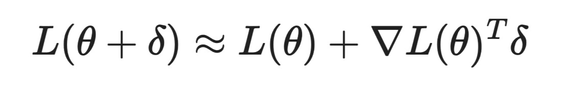
Taylor-reeks in optimalisatie

Dit werkt, maar negeert kromming. Als het verlieslandschap kromt, kan een eerste-orde benadering doorschieten of inefficiënte stappen nemen.

De methode van Newton verhelpt dit door de term van tweede orde mee te nemen - de Hessiaanmatrix H, die de kromming bijhoudt:

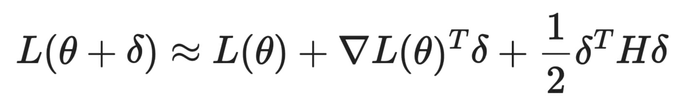
Taylor-reeks in optimalisatie (2)

De afgeleide van deze uitdrukking op nul zetten geeft je de optimale stap om te nemen. De keerzijde is dat het berekenen van de volledige Hessiaan duur is voor grote modellen. Methoden zoals L-BFGS benaderen hem in plaats daarvan, wat het grootste deel van het voordeel oplevert tegen een fractie van de kosten.

Benaderingen van activatiefuncties

Sommige activatiefuncties zijn duur om te berekenen. Taylor-reeksen geven je goedkopere alternatieven die voor de meeste doeleinden nauwkeurig genoeg zijn.

De sigmoïdefunctie σ(x) = 1 / (1 + e⁻ˣ) vereist het berekenen van een exponent, wat duur is. In de buurt van x = 0 is de Taylor-expansie:

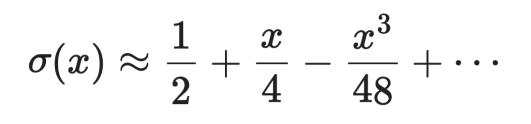
Taylor-reeks in benadering

Voor hardwarebeperkte omgevingen zoals edge devices of FPGA's kunnen zulke polynomiale benaderingen exacte berekeningen vervangen door een handvol vermenigvuldig-plus-optelbewerkingen.

GELU, gebruikt in transformermodellen zoals BERT en GPT, wordt vaak geïmplementeerd via een op Taylor gebaseerde benadering van de foutfunctie erf(x), omdat de exacte vorm een integraal bevat zonder gesloten vorm.

XGBoost en optimalisatie van tweede orde

XGBoost is een van de meest gebruikte gradient-boostingbibliotheken en gebruikt een Taylor-expansie van tweede orde van de verliesfunctie om elke nieuwe boom te fitten.

Bij elke boostingstap benadert XGBoost de loss als:

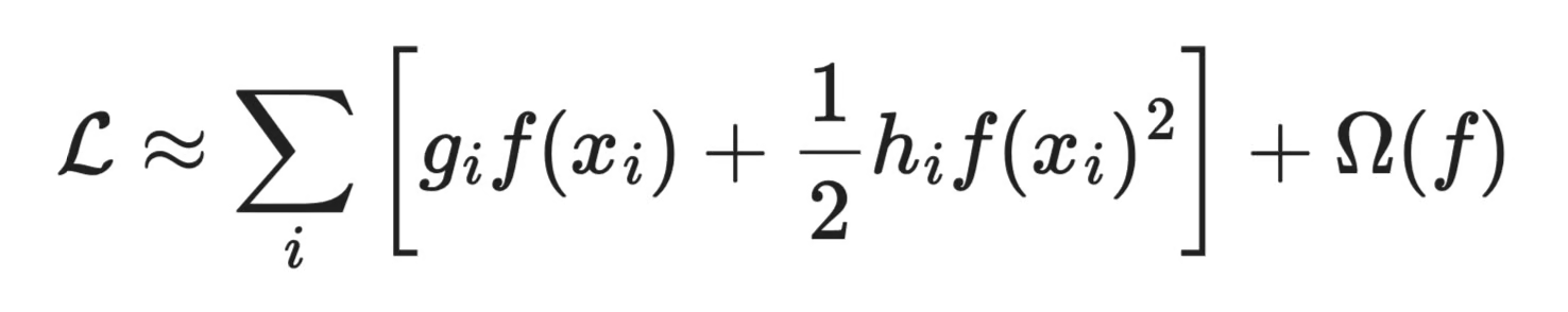
XGBoost-verliesbenadering

Waarbij g_i de gradiënt van eerste orde is en h_i de gradiënt van tweede orde (Hessiaan) van de loss ten opzichte van de huidige voorspelling. Door beide termen te gebruiken, kan XGBoost sneller en nauwkeuriger bomen fitten dan methoden van eerste orde, wat een groot deel van de goede prestaties op tabeldata verklaart.

Uitdagingen en beperkingen

Dat Taylor-reeksen overal in data science gebruikt kúnnen worden, betekent niet dat ze een metaforische hamer voor elke spijker zijn. Er kunnen een paar dingen misgaan.

• Benaderingsfout stapelt op: In diepe netwerken koppel je veel bewerkingen achter elkaar. Een kleine Taylor-benaderingsfout in één laag stapelt op over lagen, wat de trainingsstabiliteit kan beïnvloeden

• De convergentiestraal is van belang: Taylor-benaderingen zijn alleen betrouwbaar in de buurt van het uitbreidingspunt. Als je invoer ver afdrijft van waar de benadering is opgebouwd - bijvoorbeeld tijdens inferentie op out-of-distribution data - kan de benadering instorten

• Hessians in hoge dimensies zijn duur: Methoden van tweede orde zijn krachtig maar schalen niet zo goed. Een model met n parameters heeft een n × n Hessiaan. Voor een model met miljoenen parameters is het opslaan en inverteren van die matrix niet praktisch zonder benaderingen.

Als je deze afwegingen begrijpt, weet je wanneer een op Taylor gebaseerde aanpak de moeite waard is en wanneer een eenvoudigere methode van eerste orde goed genoeg is.

Bekende Taylor-reeksen

Een paar Taylor-reeksen kom je overal tegen in wiskunde, natuurkunde en machine learning. Dit zijn de reeksen die je wilt kennen als je serieus met data science bezig bent.

Exponentiële functie

De exponentiële functie eˣ is de eenvoudigste Taylor-reeks om af te leiden, omdat elke afgeleide van eˣ gelijk is aan eˣ zelf. Evaluatie bij a = 0 geeft voor elke coëfficiënt 1:

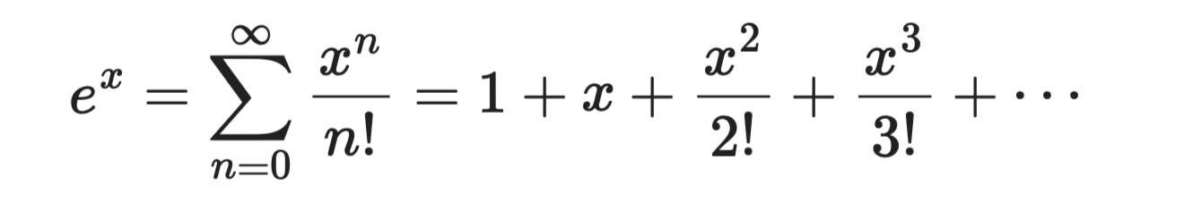
Exponentiële functie

Deze reeks convergeert voor alle waarden van x, wat haar betrouwbaar en makkelijk in gebruik maakt. Ze vormt de basis voor de sigmoid- en softmaxfuncties die in classificatiemodellen worden gebruikt.

Sinusfunctie

De sinusfunctie bevat alleen oneven machten, wat volgt uit het feit dat sin(x) een oneven functie is - dus sin(-x) = -sin(x):

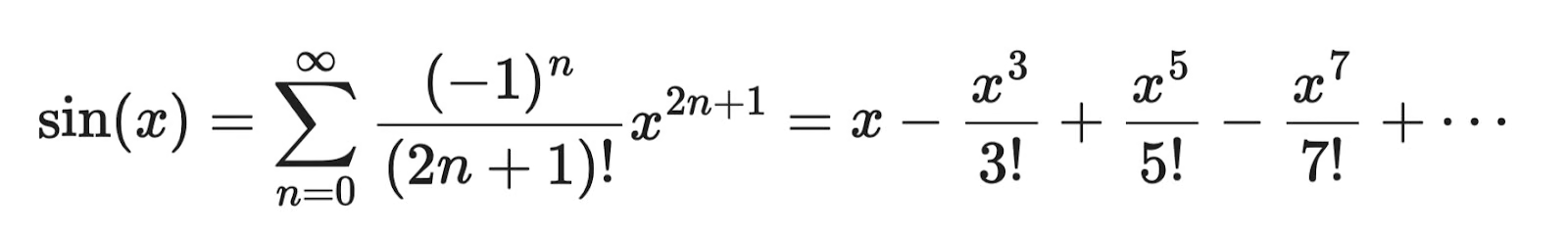
Sinusfunctie

Net als eˣ convergeert dit voor alle x. De alternerende tekens komen doordat de afgeleiden van sin(x) cycleren door cos(x), -sin(x), -cos(x) en weer terug.

Cosinusfunctie

Cosinus is de even tegenhanger van sinus - hij bevat alleen even machten:

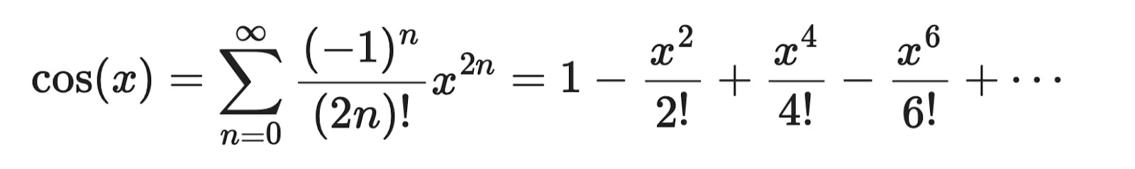
Cosinusfunctie

Als je de sinus- en cosinusreeksen naast elkaar bekijkt, valt op dat ze complementair zijn. Die relatie leidt tot Euler’s beroemde identiteit: eⁱˣ = cos(x) + i·sin(x).

Natuurlijke logaritme

De natuurlijke logaritme ln(1 + x) heeft een Taylor-reeks gecentreerd op x = 0:

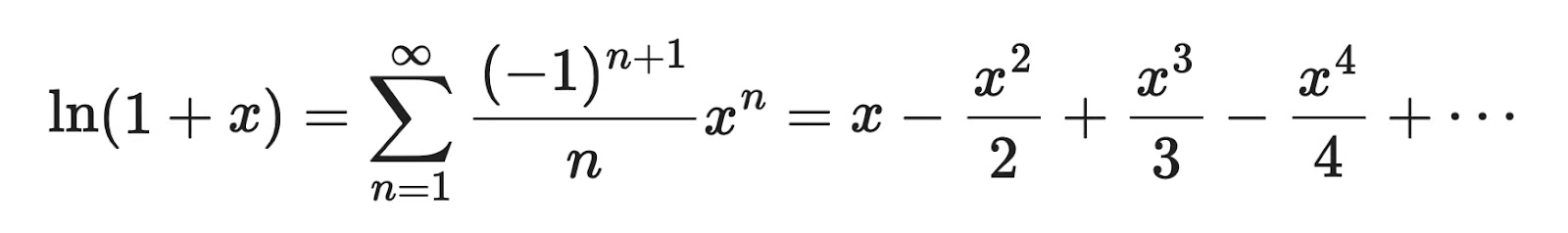
Natuurlijke logaritmefunctie

Anders dan de vorige drie convergeert deze alleen voor -1 < x <= 1. Duw je x buiten dat bereik, dan divergeert de reeks. Dit speelt bijvoorbeeld bij cross-entropy loss, waar logkansen binnen een geldig bereik moeten blijven.

Meetkundige reeks

De meetkundige reeks is een van de oudste en meest gebruikte resultaten in de wiskunde:

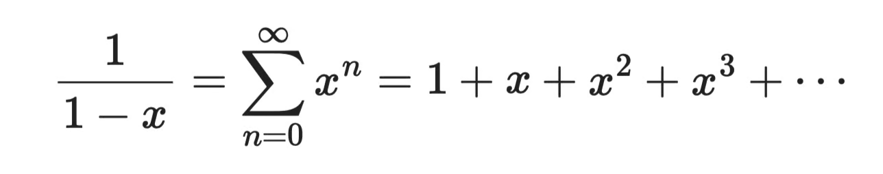
Meetkundige reeks

Deze convergeert alleen voor |x| < 1. Het is het startpunt voor het afleiden van veel andere Taylor-reeksen, en je komt hem tegen in de kansrekening, signaalverwerking en overal waar je gedisconteerde toekomstige waarden optelt.

Snel naslagwerk

Zoek je iets tastbaars, printbaars, om aan de muur naast je bed te hangen? Dan ben je gedekt:

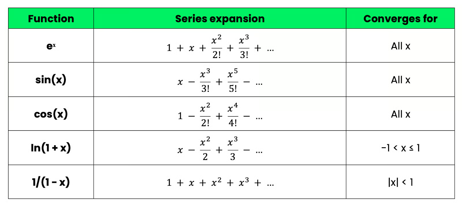
Taylor-reeksen snel naslagwerk

Deze vijf reeksen dekken het merendeel van de gevallen die je in data science en machine learning tegenkomt.

Taylor-reeksen versus andere gerelateerde reeksen

Taylor-, Fourier- en Maclaurin-reeksen benaderen allemaal functies, maar lossen verschillende problemen op en werken het best in verschillende contexten.

Taylor-reeksen vs. Fourier-reeksen

Taylor- en Fourier-reeksen representeren beide functies als oneindige sommen, maar doen dat op totaal verschillende manieren.

Een Taylor-reeks bouwt een functie op uit polynomen - machten van (x - a). Ze zoomt in op één punt en vangt het lokale gedrag van de functie via haar afgeleiden. Het resultaat is nauwkeurig in de buurt van het centrumpunt a, maar de nauwkeurigheid neemt af naarmate je ervan weg beweegt.

Een Fourier-reeks gebruikt sinussen en cosinussen als bouwstenen:

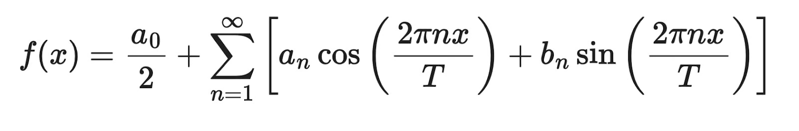
Fourier-reeks

In plaats van lokaal gedrag in één punt te vangen, leggen Fourier-reeksen globaal periodiek gedrag vast over een hele interval. Ze zijn ontworpen voor functies die zich herhalen - denk aan audiosignalen, seizoenspatronen of alles wat oscilleert.

Zo verhouden de twee zich naast elkaar:

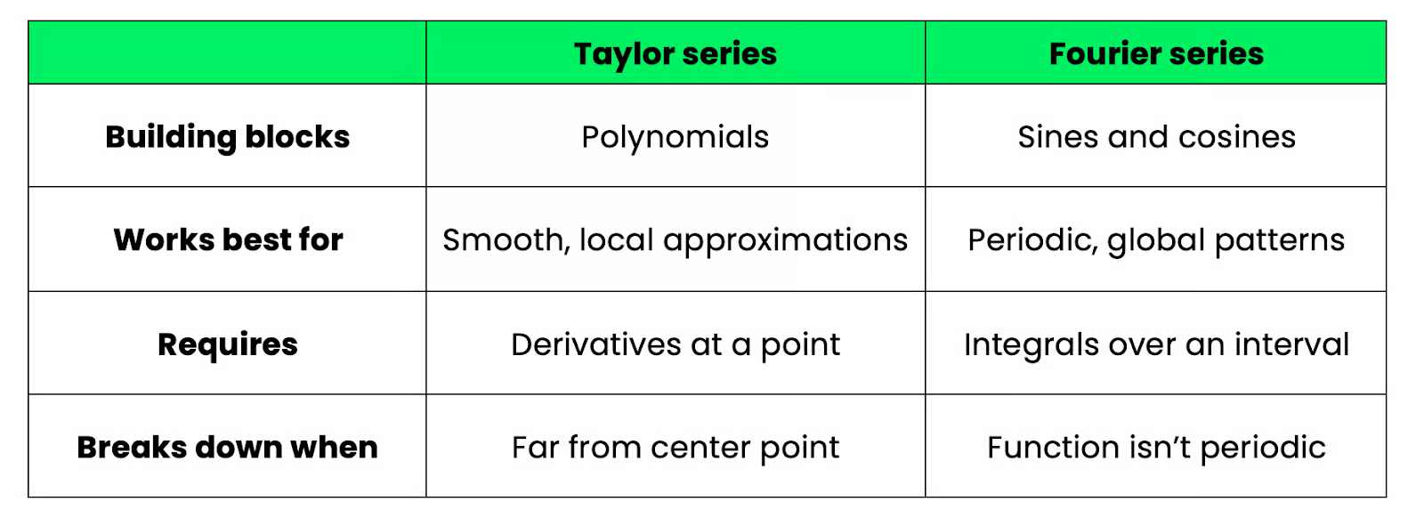
Vergelijking Taylor vs. Fourier

Fourier-reeksen kom je tegen in signaalverwerking en tijdreeksanalyse - spectrale analyse, frequentie-decompositie, en zelfs sommige neurale netwerkarchitecturen zoals FNet, dat aandacht vervangt door Fourier-transformaties.

Werk je met tabeldata, afbeeldingen of optimalisatie, dan zijn Taylor-reeksen het meest relevant. Werk je met audio, tijdreeksen of iets met periodieke structuur, dan passen Fourier-reeksen beter.

Taylor-reeksen vs. Maclaurin-reeksen

Deze is eenvoudig. Een Maclaurin-reeks is gewoon een Taylor-reeks gecentreerd op a = 0.

De algemene Taylorreeks-formule is:

Maclaurin-reeks

Zet a = 0 en je krijgt:

Maclaurin-reeks bij a = 0

Colin Maclaurin gebruikte dit specifieke geval zo vaak in zijn werk dat het een eigen naam kreeg, maar wiskundig is het niets meer dan een Taylor-reeks met een bepaald centrumpunt.

In de praktijk zijn de meeste reeksen die je ziet - eˣ, sin(x), cos(x), ln(1 + x) - Maclaurin-reeksen, omdat centreren op nul de algebra overzichtelijk houdt. Wil je een functie in de buurt van een ander punt benaderen, dan verschuif je het centrum naar a ≠ 0 en krijg je een algemene Taylor-reeks.

Kortom, elke Maclaurin-reeks is een Taylor-reeks, maar niet elke Taylor-reeks is een Maclaurin-reeks.

Taylor-reeksen en lineaire modellen

Taylor-reeksen en lineaire modellen lijken in eerste instantie misschien niet verwant, maar er is een nuttige connectie, en die begint bij de Taylor-benadering van eerste orde.

Als je een Taylor-reeks na de eerste term afkapt, krijg je een lineaire benadering van een functie bij een punt a:

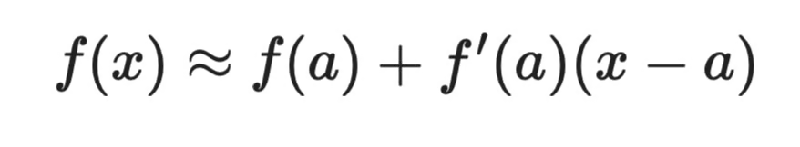
Taylor-reeksen en lineaire modellen (1)

Dit is een rechte lijn. Die heeft een helling (f'(a)) en een intercept (f(a) - f'(a) ⋅ a). Klinkt bekend? Dat is dezelfde structuur als een model voor eenvoudige lineaire regressie:

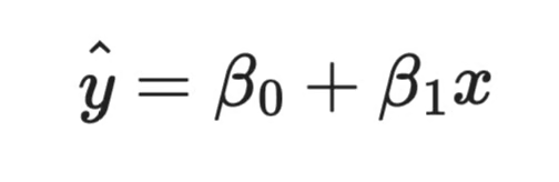
Taylor-reeksen en lineaire modellen (2)

Het verschil zit in de herkomst. In een Taylor-benadering worden helling en intercept bepaald door de afgeleiden van de functie in één punt. In lineaire regressie worden ze uit data geschat om de voorspellingsfout te minimaliseren. Maar structureel doen ze hetzelfde.

Waar deze connectie handig wordt

Het verklaart waarom lineaire modellen in bepaalde situaties goed werken en in andere niet.

Lineaire regressie gaat ervan uit dat de relatie tussen je invoer en uitvoer lineair is - of als zodanig behandeld kan worden. Taylor-reeksen vertellen je precies wanneer die aanname opgaat - wanneer je invoer dicht bij een vast punt blijft en de functie die je benadert vloeiend is. Duw je je invoer ver van dat punt af, dan breekt een lineaire benadering, om dezelfde reden dat lineaire regressie vaak faalt op data met sterke niet-lineaire patronen.

Generalized linear models (GLM's) maken deze connectie nog explicieter.

Logistische regressie bijvoorbeeld modelleert de log-odds van een uitkomst als een lineaire functie. De koppeling tussen de lineaire voorspeller en de uitvoerkans loopt via de sigmoïdefunctie - en zoals je eerder zag, heeft de sigmoïde een goedgedragende Taylor-expansie nabij nul.

Van lineair naar niet-lineair

Zodra je begrijpt dat een Taylor-expansie van eerste orde je een lineair model geeft, is de volgende stap om meer termen op te nemen, en krijg je een polynoommodel.

Een Taylor-expansie van tweede orde geeft je:

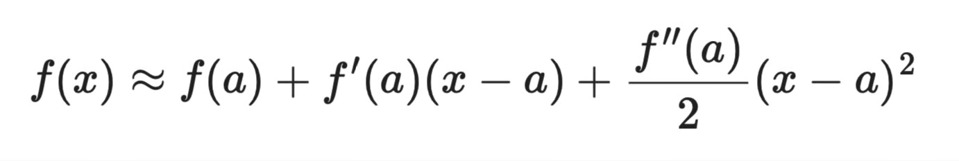
Taylor-reeks van tweede orde

Dit is een kwadratische term - een polynomiale regressie met een kwadraatterm. Elke extra Taylor-term correspondeert met een polynoom van hogere graad, en zo breidt polynomiale regressie lineaire regressie uit om gekromde relaties te vangen.

Taylor-reeksen geven je dus een onderbouwde manier om na te denken over de bias-variantieafweging in regressie. Een benadering van eerste orde (lineair model) is snel en interpreteerbaar maar heeft hoge bias als de werkelijke relatie niet-lineair is. Hogere-orde benaderingen passen de data beter in de buurt van het uitbreidingspunt, maar lopen meer risico op overfitting naarmate je termen toevoegt.

Wil je dieper in lineaire regressie en wanneer die werkt, dan is de tutorial Essentials of Linear Regression in Python een goed vervolg. Voor R-gebruikers behandelt de cursus Intermediate Regression in R polynomiale regressie en modeldiagnostiek in detail.

Conclusie

Taylor-reeksen zijn van die wiskundige hulpmiddelen die je overal ziet zodra je weet waar je op moet letten.

Je hebt gezien hoe ze computers functies als eˣ en sin(x) laten uitrekenen via basisrekenwerk, hoe convergentie en afsnijfout bepalen hoe nauwkeurig een benadering is, en hoe hetzelfde idee gradient descent, XGBoost en benaderingen van activatiefuncties in moderne machine learning aandrijft.

De vijf bekende reeksen - exponentieel, sinus, cosinus, logaritmisch, meetkundig - zijn het waard om te onthouden. Je komt ze vaak genoeg tegen dat ze herkennen op het oog echt tijd scheelt.

Van hieruit is de volgende stap om comfortabel te worden met het algoritmisch denken dat naast dit soort wiskunde hoort. Onze cursus Data Structures and Algorithms in Python is een solide plek om die basis te leggen. Het helpt je te begrijpen hoe wiskundige ideeën vertalen naar code die werkt en schaalt.