As it turns out, you're using the results of differential equations every time you train a neural network or even fit a regression model. The math running underneath is calculus, and differential equations sit right at the center of it. If you've ever wondered why gradient descent works, or how a Kalman filter tracks a moving object, differential equations are your answer.
Differential equations let you model how things *change over time* - and that's exactly what data science is about. Once you understand the core ideas, you'll start seeing them everywhere: in the loss functions you minimize, the time series you forecast, and the simulations you run.
In this article, I'll walk you through what differential equations are, the main types you'll see, how to solve them, and - most importantly - how they show up in real data science and machine learning day to day.
What Are Differential Equations?
A differential equation is an equation that relates a function to its own derivatives.
In plain terms, a derivative tells you how fast something is changing at a given moment. A differential equation says that the rate of change of a quantity depends on the quantity itself, or on time, or on both.
Say you're modeling a population of bacteria. The more bacteria you have, the faster they reproduce. So the growth rate depends on the current population size. Write that as an equation, and you've got a differential equation.
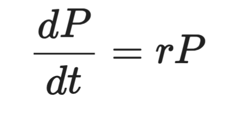
Formally, it looks like this:
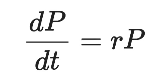
Differential equation representation
Where P is the population, t is time, and r is the growth rate. The left side is the derivative - how fast P changes over time. The right side says that change is proportional to P itself.
That's the core idea behind every differential equation you'll see.
Differential equations show up across physics, biology, and engineering - anywhere a system evolves over time. Heat spreading through a metal rod, a pendulum swinging, a virus spreading through a population. All of these are modeled with differential equations.
For data scientists, you’ll see differential equations in loss functions, gradient descent, time series models, neural ODEs - they all have differential equations running underneath. You don't always see them explicitly, but they're there.
When you understand them, you’ll have a clearer mental model of why and how the tools you use every day work.
The History of Differential Equations
In the late 17th century, Isaac Newton and Gottfried Wilhelm Leibniz independently developed calculus. Both needed a way to describe how physical quantities change over time, and differential equations were the result. Newton used them to model motion and gravity. Leibniz gave us much of the notation we still use today, including the d/dt you'll see in every calculus textbook.
The 18th and 19th centuries brought a wave of new techniques.
Leonhard Euler developed methods for solving ODEs numerically - the same Euler behind Euler's method you'll see later in this article. Joseph-Louis Lagrange and Pierre-Simon Laplace extended the theory to more complex systems. Jean-Baptiste Joseph Fourier introduced a way to decompose functions into sine and cosine components, which became a cornerstone of solving partial differential equations.
By the 20th century, differential equations were everywhere from fluid dynamics, quantum mechanics, to electrical engineering. Many real-world equations had no clean analytical solution. That's where numerical methods took over, and computers made them practical at scale.
Today, the field keeps moving. Neural ordinary differential equations (Neural ODEs) treat the layers of a neural network as a continuous process described by a differential equation. It's a recent development that blurs the line between deep learning and classical mathematics. It’s also and it's one of the more exciting areas in modern ML research.
That said, the core idea stays the same: model how things change, and you can predict where they're going.
Types of Differential Equations
Not all differential equations are the same. The first thing you need to know is how to tell them apart.
The main split is between ordinary differential equations (ODEs) and partial differential equations (PDEs). The difference comes down to how many independent variables the function depends on.
Ordinary differential equations (ODEs)
An ordinary differential equation involves a function of a single independent variable and its derivatives.
The bacteria population example from earlier is an ODE. The population P depends only on time t - one variable. So the equation only has ordinary derivatives, written as dP/dt.
ODEs are the right tool when your system evolves along a single dimension, usually time. Here’s a couple of classic examples:
- Population growth - the rate of change of a population depends on the current population size
- Radioactive decay - the rate at which a substance decays depends on how much of it remains
- Newton's second law - the acceleration of an object depends on the forces acting on it
In each case, one variable drives the change. That's what makes it ordinary.
Partial differential equations (PDEs)
A partial differential equation involves a function of multiple independent variables and its partial derivatives.
Say you want to model how heat spreads through a metal rod. The temperature at any point depends on both where you are along the rod and what time it is. That's two independent variables: position x and time t. When you write an equation for that, you get partial derivatives - one with respect to x, one with respect to t.
That's a PDE. The heat equation is one of the most well-known examples:
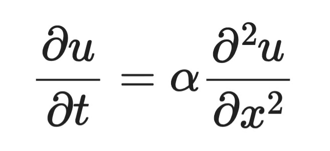
Partial differential equation example
Where u(x, t) is the temperature at position x and time t, α is the thermal diffusivity of the material, ∂u/∂t is how fast temperature changes over time, and ∂²u/∂x² is how curved the temperature profile is across space. The equation says that where the temperature curve bends sharply, heat redistributes fast. Where it's flat, not much happens.
PDEs show up wherever a system varies across space and time:
- Heat distribution - temperature changes across both position and time
- Wave propagation - sound or light waves spread across space over time
- Fluid dynamics - fluid velocity depends on position in 3D space and time
PDEs are harder to solve than ODEs. Analytical solutions exist only for specific forms, and numerical methods are often the only practical path forward.
For most data science work, you'll encounter ODEs more often. But PDEs appear in image processing, physics simulations, and some deep learning architectures, so you need to know the differences.
Order and Degree of Differential Equations
Every differential equation has two properties that tell you how complex it is: its order and its degree.
These determine which solution methods apply, so you need to identify them before you try to solve anything.
Understanding order
The order of a differential equation is the order of the highest derivative in the equation.
If the highest derivative is a first derivative (dy/dx), it's a first-order equation. If the highest is a second derivative (d²y/dx²), it's a second-order equation. And so on.
Here’s the bacteria growth equation from earlier:
Bacteria growth equation
The highest derivative here is dP/dt - a first derivative. So this is a first-order ODE.
Now compare that to the equation describing a swinging pendulum:
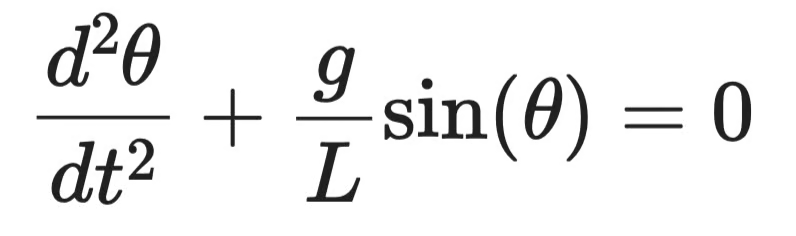
Swinging pendulum equation
The highest derivative is d²θ/dt² - a second derivative. That makes it a second-order ODE.
Higher order means more complexity. Second-order equations need two initial conditions to solve instead of one. In practice, most physical systems - mechanical motion, electrical circuits, orbital dynamics - are modeled with second-order equations.
Understanding degree
The degree of a differential equation is the power of the highest-order derivative, once the equation is written in a polynomial form (no radicals or fractions involving derivatives).
Take this equation:
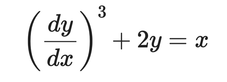
Sample differential equation
The highest derivative is dy/dx, and it's raised to the power of 3. So the order is 1 and the degree is 3.
Now take this one:
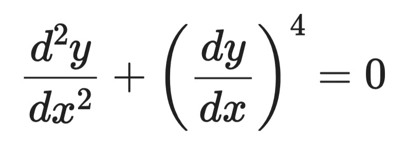
Sample differential equation (2)
The highest-order derivative is d²y/dx², raised to the power of 1. The degree is 1, even though a lower-order derivative appears with a higher power.
The degree always follows the highest-order derivative, not the highest power in the equation.
One edge case is if an equation contains terms like sin(dy/dx) or e^(d²y/dx²). Then, the degree is undefined - those forms can't be expressed as polynomials in the derivatives.
Methods for Solving Differential Equations
There's no single method that works for every differential equation. The right approach depends on the equation's type, order, and whether an exact solution even exists.
Broadly, you've got two categories: analytical methods and numerical methods.
Analytical methods
Analytical methods give you an exact, closed-form solution - a formula you can evaluate at any point. They're preferred when they apply because the result is precise and tells you something about the structure of the solution.
But they only work for specific equation forms. When the equation gets too complex, analytical methods hit a wall.
Separation of variables
Separation of variables works on equations where you can isolate all terms involving y on one side and all terms involving x (or t) on the other.
Take this first-order ODE:
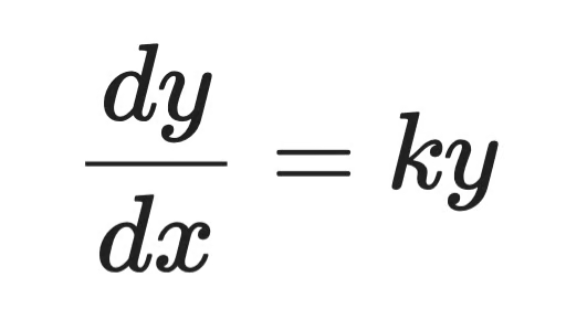
Simple differential equation
Step 1 - separate the variables:
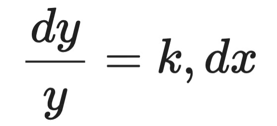
Analytical solution (step 1)
Step 2 - integrate both sides:
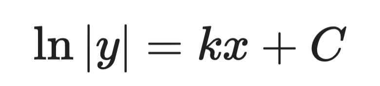
Analytical solution (step 2)
Step 3 - solve for y:
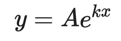
Analytical solution (step 3)
Where A is a constant determined by initial conditions. That's the general solution.
This is the same form as the bacteria growth equation. It tells you that populations - and anything else with a growth rate proportional to its size - grow exponentially.
Integrating factors
Integrating factors handle first-order linear ODEs of this form:
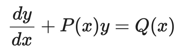
Integrating factors example (1)
The idea is to multiply both sides by a carefully chosen function - the integrating factor μ(x) - that makes the left side a perfect derivative you can integrate directly.
The integrating factor is always:
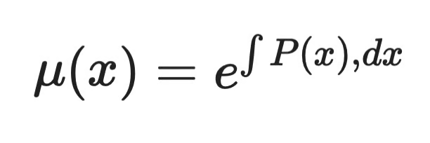
Integrating factors example (2)
After multiplying through, the equation becomes:
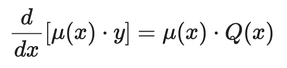
Integrating factors example (3)
Then integrate both sides and solve for y. The left side always collapses cleanly because of how μ(x) was chosen - that's the whole point of the method.
Numerical methods
Most real-world differential equations don't have clean analytical solutions. Numerical methods approximate the solution step by step, computing values at discrete points.
They trade exactness for generality. And in practice, that's often exactly what you need.
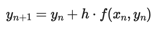
Euler's method
Euler's method is the simplest numerical approach. The idea is to start at a known point, use the derivative to estimate the slope, take a small step in that direction, and repeat.
Given a first-order ODE dy/dx = f(x, y) with initial condition y(x₀) = y₀, each step looks like:
Euler’s method example (1)
Where h is the step size. Smaller steps mean better accuracy - but more computation.
Here's a Python implementation solving dy/dx = y with y(0) = 1 (the exact solution is y = eˣ):
import numpy as np
import matplotlib.pyplot as plt

def euler_method(f, x0, y0, h, n_steps):
    x = np.zeros(n_steps + 1)
    y = np.zeros(n_steps + 1)
    x[0], y[0] = x0, y0

    for i in range(n_steps):
        y[i+1] = y[i] + h * f(x[i], y[i])
        x[i+1] = x[i] + h

    return x, y

f = lambda x, y: y  # dy/dx = y

x_euler, y_euler = euler_method(f, x0=0, y0=1, h=0.2, n_steps=20)
x_exact = np.linspace(0, 4, 200)
y_exact = np.exp(x_exact)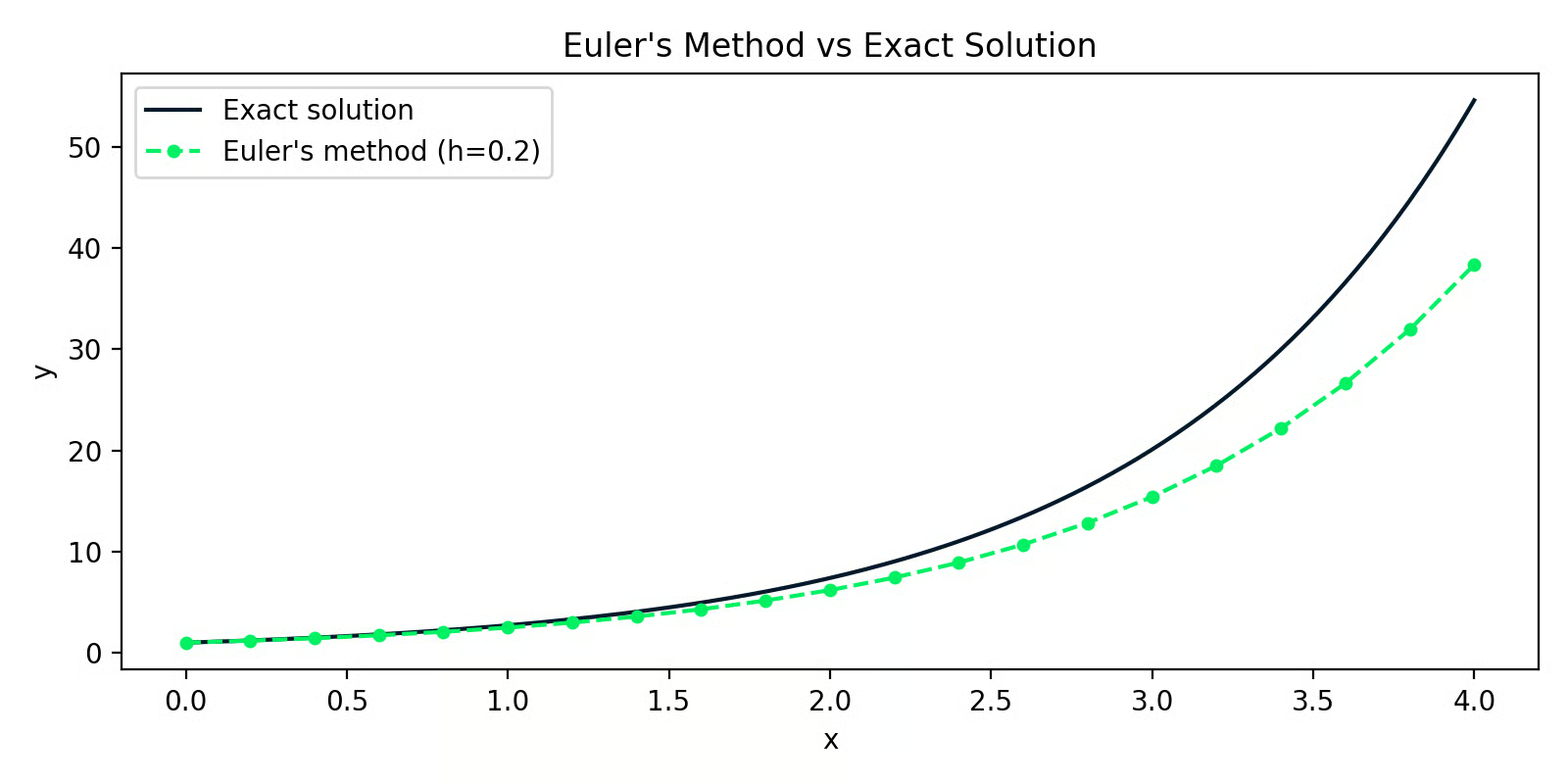
Euler's method versus the exact solution
The gap between the two lines is the approximation error. With h=0.2, the error is small at first but compounds over steps - that's the main weakness of Euler's method.
Runge-Kutta methods
Runge-Kutta methods fix that compounding error problem by sampling the slope at multiple points within each step and taking a weighted average. The most common version is RK4 - the fourth-order Runge-Kutta method.
Instead of one slope estimate per step like Euler, RK4 computes four:
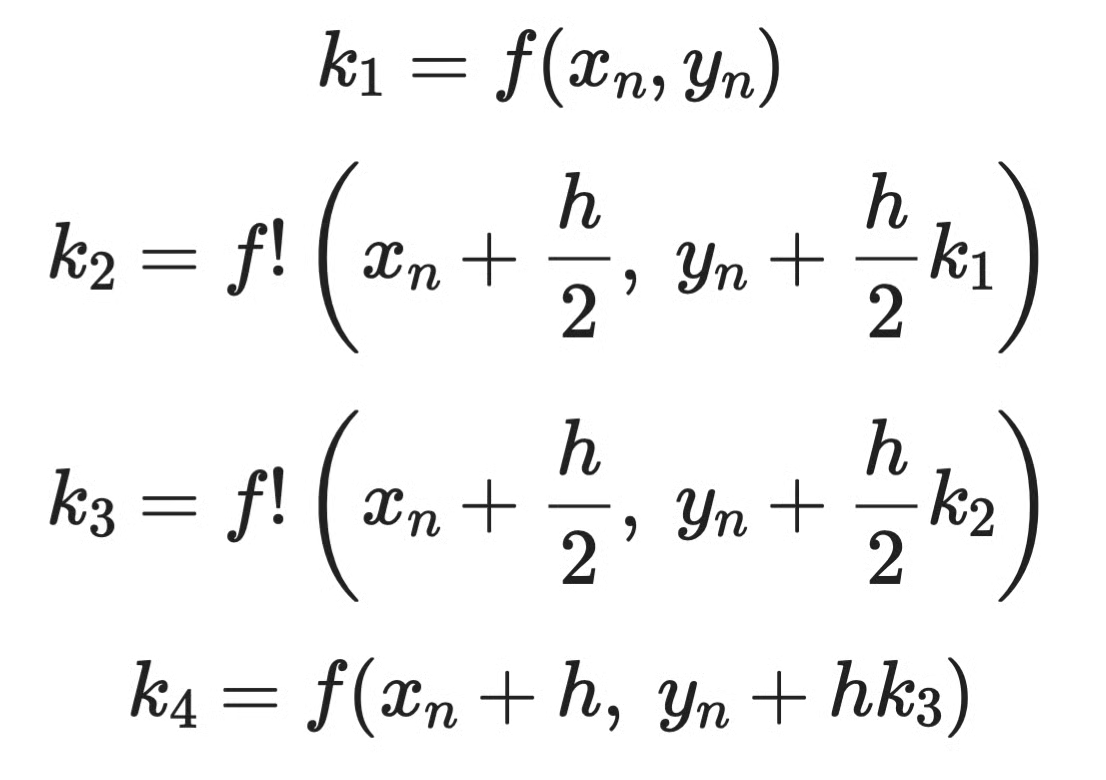
Runge-Kutta method example (1)
Then combines them:
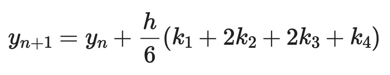
Runge-Kutta method example (2)
In practice, you don't implement RK4 by hand. SciPy's solve_ivp handles it for you:
from scipy.integrate import solve_ivp
import numpy as np
import matplotlib.pyplot as plt

f = lambda x, y: y  # dy/dx = y

sol = solve_ivp(f, t_span=[0, 4], y0=[1], max_step=0.2)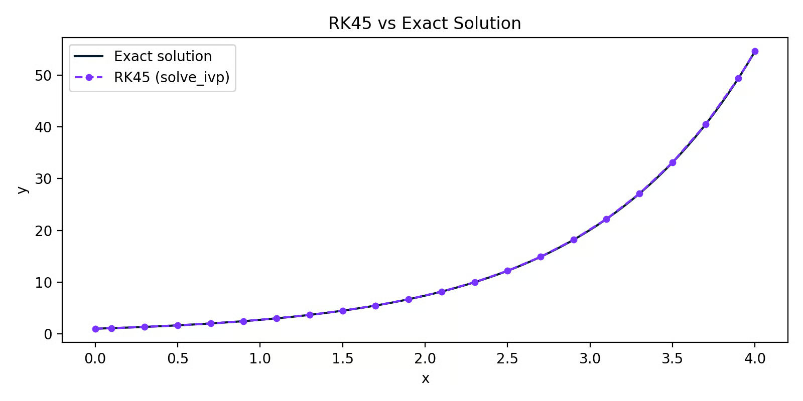
RK45 versus the exact solution
The RK45 line sits almost perfectly on top of the exact solution. Same step size as the Euler example, but far better accuracy - that's the difference weighted slope sampling makes.
For most practical work in Python, solve_ivp with the default RK45 solver is your go-to. Euler's method is useful for understanding how numerical solvers work, but you wouldn't use it in production.
Applications of Differential Equations in Data Science and Machine Learning
Engineers use differential equations to model electrical circuits and mechanical systems. Biologists use them to track population dynamics and disease spread. Physicists use them to describe everything from heat transfer to quantum mechanics.
But you're here for data science, so let's get to that.
Machine learning and optimization
The most direct connection between differential equations and ML is gradient descent - the algorithm behind training nearly every model you'll build.
When you train a model, you're minimizing a loss function L. To do that, you need to know how L changes as you adjust each parameter. That rate of change is a derivative. When your model has multiple parameters, you compute a partial derivative for each one - and together, they form the gradient.
Gradient descent uses those derivatives to update parameters step by step:
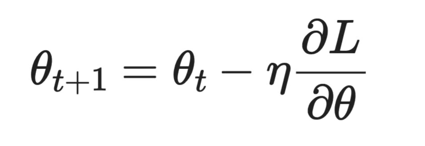
Gradient descent
Where θ is the parameter, η is the learning rate, and ∂L/∂θ is the partial derivative of the loss with respect to that parameter.
Here's a simple Python example fitting a line to data using gradient descent:
import numpy as np
import matplotlib.pyplot as plt

np.random.seed(42)
X = np.linspace(0, 10, 100)
y = 2.5 * X + np.random.randn(100) * 2

# Initialize parameters
theta = 0.0
bias = 0.0
eta = 0.001
n = len(X)
losses = []

for _ in range(500):
    y_pred = theta * X + bias
    loss = np.mean((y_pred - y) ** 2)
    losses.append(loss)

    # Partial derivatives
    d_theta = (2/n) * np.sum((y_pred - y) * X)
    d_bias  = (2/n) * np.sum(y_pred - y)

    theta -= eta * d_theta
    bias  -= eta * d_bias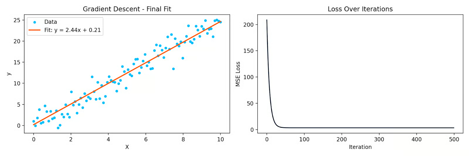
Gradient descent fitting a line to data, and the loss curve over iterations
Each iteration moves the parameters in the direction that reduces the loss. The partial derivatives tell you which direction that is. Without them, gradient descent doesn't work - and neither does backpropagation in neural networks, which is just the chain rule applied repeatedly through layers.
Time series analysis
Many time series systems are dynamic - the current value depends on past values and how fast things are changing. Differential equations allow you to describe that.
The Kalman filter, widely used in tracking and forecasting, is built on a system of differential equations that model how a hidden state evolves over time and how noisy observations relate to that state. It's used in GPS systems, finance, and weather forecasting.
ARIMA models are used for time series forecasting, and connect to differential equations through the concept of differencing. Taking first or second differences of a time series is a discrete approximation of first and second derivatives. When you differentiate a series to make it stationary, you're asking: how is this series changing over time?
Statistical modeling and regression
Here's one that often surprises people: solving a system of differential equations is one way to derive linear regression coefficients.
When you fit a linear regression model, you're minimizing the sum of squared residuals. Take the partial derivative of that loss with respect to each coefficient, set them to zero, and solve. That gives you the Normal Equation:
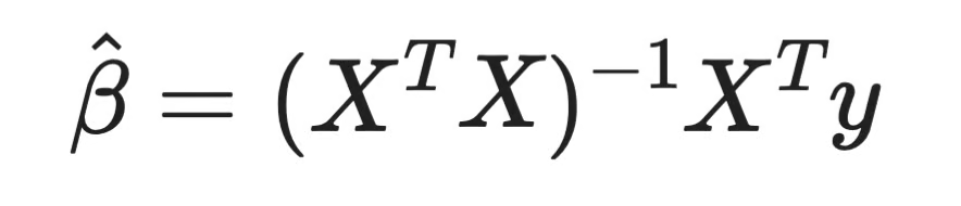
Normal equation
Every regression coefficient you've ever computed came from setting a derivative to zero and solving. That's calculus - and it's the same principle behind every parametric model you fit.
For logistic regression, the loss function isn't quadratic, so there's no closed-form solution. You have to use iterative methods like gradient descent, which, again, relies on partial derivatives at every step.
The connection goes further. QR decomposition, one of the standard numerical methods for solving the Normal Equation, is grounded in linear algebra that intersects directly with how systems of equations - including differential ones - are solved in practice.
Simulation of dynamic systems
When you need to model how a system evolves over time - and an analytical solution doesn't exist - you simulate it numerically.
This is common in business and operations contexts. Customer churn, inventory levels, and supply chain dynamics all involve quantities that change based on the current state. You can write those relationships as differential equations and simulate them with solve_ivp.
Here's an example simulating a simple supply-demand system where inventory I depletes at a rate proportional to demand D, and demand shifts over time:
import numpy as np
from scipy.integrate import solve_ivp
import matplotlib.pyplot as plt

def supply_chain(t, y):
    I, D = y
    dD_dt = 0.1 * np.sin(0.5 * t)   # demand fluctuates over time
    dI_dt = -D                      # inventory depletes at the demand rate
    return [dI_dt, dD_dt]

sol = solve_ivp(
    supply_chain,
    t_span=[0, 20],
    y0=[100, 5],  # initial inventory=100, demand=5
    max_step=0.1
)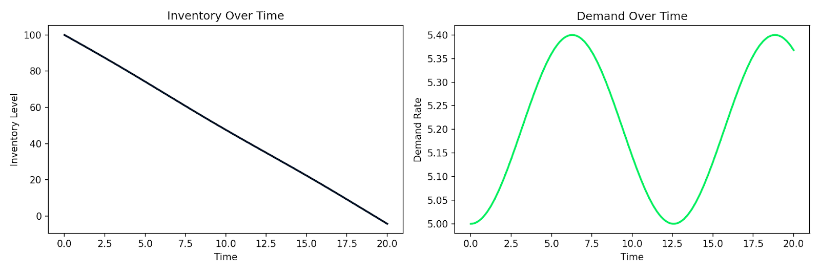
Simulated inventory depletion alongside fluctuating demand over time
The same pattern applies to customer behavior modeling, epidemic spread in a user base, or any system where the rate of change depends on the current state. You write down the relationships, hand them to a numerical solver, and get a simulation back.
And that's the practical power of differential equations in data science. It’s a direct tool for modeling systems that change.
Conclusion
Behind gradient descent, there are partial derivatives. Behind time series forecasting, there are dynamic systems. Behind linear regression coefficients, there are derivatives set to zero. You just need to know where to look.
In this article, I explained what differential equations are, the difference between ODEs and PDEs, how order and degree classify them, and the main methods for solving them - both analytical and numerical. Then we looked at where they actually show up in data science and machine learning day to day.
This is just the foundation. If you want to explore more math topics, Linear Algebra for Data Science in R course is a good next step. For hands-on practice applying these concepts to real data problems, check our Quantitative Analyst in R course.