
Cursus
Lineaire algebra voor data science in R
4 Hr
21K
Aspiring and junior data scientists often see the term "function" used, but it's not always clear what the term actually means.
In this article, you will learn what a mathematical function is, which sets describe its input and output values, and how continuous and discrete values differ. You'll explore how functions are used in technology, common functions in data science, and how they are optimized. Along the way, you will see Python code to manipulate and plot functions.
If you want to practice writing and using your own functions in Python, I recommend taking our Writing Functions in Python course.
In mathematics, a function maps each input to a unique output. Each valid input is sent to one and only one output. An input can't somehow have multiple outputs.
For instance, 32 degrees Fahrenheit is 0 Celsius. The Fahrenheit value corresponds to a value in Celsius; it also corresponds to only one value. You can't have two different output values (Celsius) for one valid input (Fahrenheit).
Other examples include payroll, where you are paid an amount per hour. If you make $20 an hour and work 40 hours, you make 20 x 40 = $800.
Not all rules are functions. In some cases, it makes logical sense to have multiple outputs for a single input. For instance, matching a name to a person is not a function. The name "John Smith" could map to a number of people, all of whom share this name.
In mathematics, rules are often set up in such a way that there is only one output per valid input. In many cases, this is explicitly how the world really works (payroll). In other cases, problems are formulated in terms of functions because they make the problem tractable. Rather than following a spaghetti tangle of inputs and outputs, the model is set up in such a way that each input cannot have multiple outputs.
You can think of a function as a "machine" that accepts an input (often denoted x), processes it in some way, and outputs an output (often denoted y).
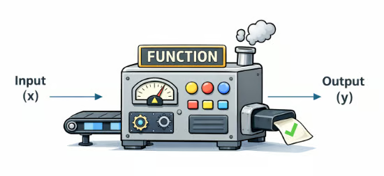
Here, a machine accepts input from its conveyor belt on the left-hand side, processes it, and produces a cheerful green check mark on the right.
Multivariate functions accept a collection of multiple inputs but only output one output. You can think of this as passing in one row of data that consists of several variables or features that map to a single output.
How do you write down the equation? In the temperature conversion example, we could write the formula as y = f(x) = (5/9) (x - 32), with x being the temperature in Fahrenheit and y in Celsius. To understand this notation, parse it from left to right.
On the left, you see y, which is the output. The notation f(x) indicates that you are using a function, called f, that takes an input x. Note that in this context, f(x) does not mean some value f multiplied by some other value x.
On the right is the formula. It says to take the input x, subtract 32 from it, and multiply this result by 5/9.
Suppose you record the outdoor temperature once a day and have collected k measurements, denoted (x1, x2, …, xk). You want a function that returns the year-to-date average temperature after n days have passed. Define a function that takes a positive integer n less than or equal to k that returns the average of the first n temperatures, which is a real number. The notation for such a function is f: {1, 2, …, k} → ℝ.
It is helpful to have jargon to describe the sets in the function, which leads us to the domain, codomain, and range.
Now, let's look at the range. Consider a simple quadratic function: y = f(x) = x2. To specify the domain and codomain, write f: ℝ → ℝ.
Now you know that this indicates that both the domain (set of inputs) and the codomain (set of outputs) consist of real numbers. However, with some thought, you might realize that the set of outputs cannot be all of the real numbers.
Since any number squared is non-negative, the set of outputs that are actually realized isn't all of the real numbers, but only non-negative real numbers. The term to describe this situation is range. We say the range of this function is all non-negative real numbers.
The codomain is the potential output set; the range is the set of actual outputs. You choose the codomain to reflect the type of output you intend, and you discover the range, which is the set of output values that are actually realized.
This brings us to the distinction between continuous and discrete variables:
For instance, a continuous variable in [0, 1] could take on the values 0, 0.5, 0.4141, or any other real value in the range. Continuous variables are commonly used in models where the output could theoretically be any value, such as in regression.
However, in binary classification, you only care about two values: 0 and 1. For instance, a picture either contains a cat or it doesn't. In a multi-class classification problem, you still only have a finite number of values, say 0 for a dog, 1 for a cat, 2 for a horse.
The problem you are trying to solve dictates what kind of function you're interested in. Classification problems yield discrete values; regression problems yield continuous functions.
Sometimes you need to pass multiple variables into a function. For instance, you might pass a row of features into a machine learning function. In this case, you can group the features into one container and pass that in. One way to group data into a container this way is via a vector. The model takes an input vector x = [x1, x2, x3] and outputs a target y.
In Python, you typically use a NumPy array to represent a vector.
import numpy as np

def f(x):
    result = (x[0] + x[1] + x[2]) / 3
    return result

x = [3, 4, 7.1]
print(f(x))4.7This code takes a vector consisting of the numbers 3, 4, and 7.1 and returns an average.
For a collection of vectors, one popular method is to use the DataFrame data structure from the pandas library.
import pandas as pd

def row_averages(df):
    return df.mean(axis=1).round(1)

df = pd.DataFrame({
    "A": [1, 5, 2],
    "B": [9, 3, 6],
    "C": [7, 8, 10]
})

print(row_averages(df))
This code returns a pandas Series containing the row averages, one value per row. In this case:
0    5.7
1    5.3
2 6.0The concept of function is ubiquitous in technology. For practical reasons, be aware that "function" is not always defined as rigorously in technology as in mathematics. For instance, programming functions can have side effects that change the values of variables other than the output, while mathematical functions don't.
Functions are used widely in spreadsheets, for example, in Excel Formulas. You might want to calculate the sum, the mean, or the median of a column of numbers. For spreadsheets, functions follow the same definition as the mathematical one introduced earlier.
One thing spreadsheets excel at (pun intended) is Conditional Functions: They allow you to build more complex conditional structures using functions like IF().
For instance, you might want to find the total of payments made to your mortgage company during a year. To do so, you'd likely use the SUM() function of your spreadsheet.
Functions are ubiquitous in programming languages. Depending on the programming language, the definition of "function" might be looser than that of a mathematical function. Some languages allow a function to return multiple values, or no value at all.
For instance, a function might take values and print a statement, but not explicitly return a value. A Python Function looks like this:
def print_me(name, color):
       print(f"My name is {name} and my favorite color is {color}.")

name = "Mark"
color = "blue"
print_me(name, color)
This code results in the output: "My name is Mark and my favorite color is blue." No mathematical value is explicitly returned from the function.
Code in many mainstream languages, such as Python, might also have other side effects in a function, such as changing the value of a global variable. Even though side effects are possible and allowed, they are discouraged. Side effects make programs more difficult to test, debug, and think through.
For these reasons, some "functional" languages, such as Scala and Haskell, are more rigorously based around the idea of a function.
In a Machine Learning context, the inputs are features, the function is the model, and the output is the model's prediction. Such a model is often described as a "black box" because it is not necessarily clear how the input features were processed to give the output prediction, which is why our earlier ”machine” metaphor fits even better:
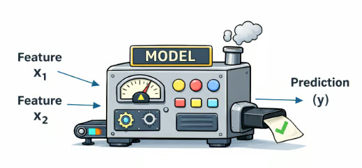
In this illustration, the features are fed into the model "machine", which processes them in some way and outputs a prediction. Compared to simpler, deterministic functions like the temperature conversion example, what happens inside the machine is harder to describe.
In ML, the domain is feature vectors; the codomain might be probabilities, classes, or real-valued predictions.
In the area of Deep Learning, functions are usually not directly applied to a set of inputs, but the correctness of the model is assessed using a cost function. A Cost Function is a measure of how wrong a model is across the training set. It compares predictions to true labels or values and aggregates the errors into a single number.
Certain functions appear almost everywhere in data science. These functions include linear functions, logarithmic functions, and exponential functions, as well as non-linear activation functions for deep learning.
Let’s start with the classic example, linear functions.
Suppose you are hungry for apples. You go to a grocery store that sells apples at a fixed price of $0.75 per pound. So one pound of apples costs $0.75, 2 pounds cost 2 x $0.75 = $1.50, and 3 pounds cost 3 x $0.75 = $2.25. Each pound you buy adds a fixed amount to the total cost.
In function notation, you might write the formula as f(x) = 0.75 x. The number 0.75 is the slope of the linear function. The slope is the rate of change of the output with respect to each unit change in the input.
To graph such a function, you can use code similar to the following:
import numpy as np
import matplotlib.pyplot as plt

def cost_of_apples(x, m):
    result = m * x
    return result

# Define x and y
x = np.linspace(0, 5, 100)
y = cost_of_apples(x, 0.75)

# Plot
plt.figure()
plt.plot(x, y)
plt.xlabel("Pounds of Apples")
plt.ylabel("Total Cost ($)")
plt.title("Cost of Apples")
plt.show()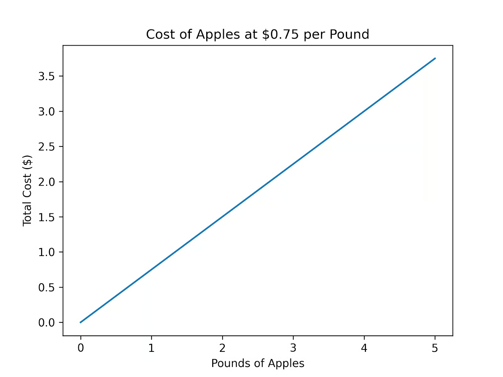
Such functions are called linear functions. Each increase in the input, x, contributes the same fixed amount to the output, y. As the name suggests, when graphed, a linear function yields a line.
Now, suppose that you like your groceries delivered. The grocery store has a flat $2.00 delivery fee. In this case, the function for your apples is f(x) = 0.75 x + 2. As before, 0.75 is the slope. The number 2, which is where the graph crosses the y-axis, is known as the "y-intercept." It is the output value when the input is 0.
The total cost is the sum of the apples and a delivery fee. In general, a univariate linear function can be written as f(x) = mx + b, where the value m is called the slope and b is called the y-intercept.
You'll probably want to eat more than just apples. Suppose you want to buy some bread and peanut butter, too. Apples cost $0.75 per pound, a loaf of bread costs $2.50, and a jar of peanut butter costs $3.00. Now, your grocery bill function is:

This function is still considered linear because it is linear in each variable. In general, a linear function takes the form:

This amounts to adding up each of your quantities multiplied by their weights (another word for slope used in this context), plus the intercept.
In vector notation, this function is written as follows:
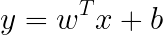
The T here stands for “transposed”, which is necessary to perform the vector multiplication for w and x.
Consider fuel efficiency versus speed. You suspect that as one drives faster, fuel efficiency decreases. You gather fifty data points between speeds of 45 and 65 miles per hour and see the following pattern:
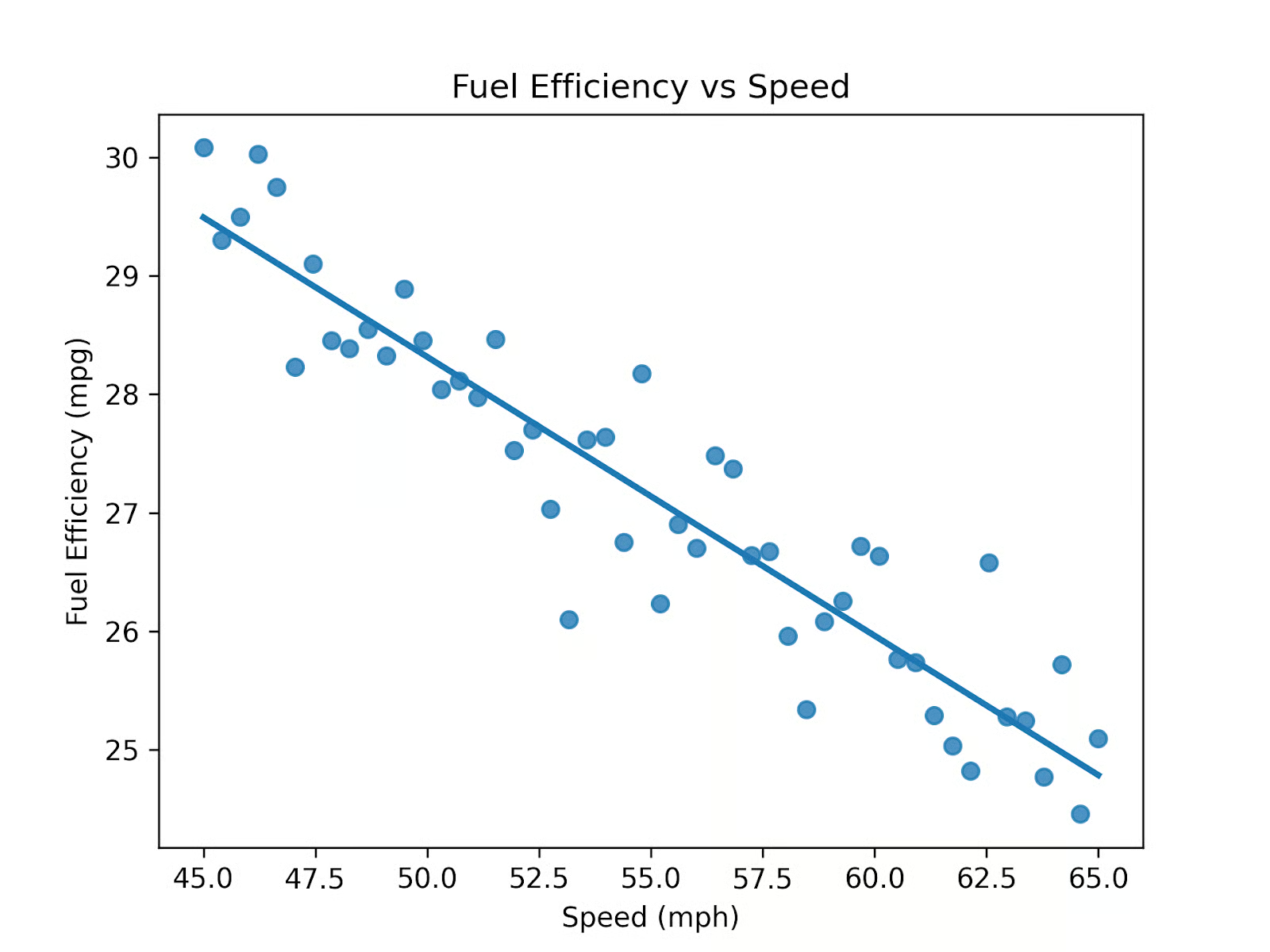
Connecting each data point would give you a squiggly, hard-to-read, unhelpful model. But the general trend of the data is approximately linear over this range. If we call speed x, the function for this graph is:
To find a line like this that best fits the data, you use a mathematical process called Simple Linear Regression.
You can compute a line like that in Python using Matplotlib and Seaborn:
import numpy as np
import pandas as pd
import seaborn as sns
import matplotlib.pyplot as plt

# Reproducibility
np.random.seed(0)

# Create dataset
speed = np.linspace(45, 65, 50)
mpg = 38 - 0.2 * speed + 0.002 * (speed - 55)**2 + np.random.normal(0, 0.5, size=50)

df = pd.DataFrame({
    "speed": speed,
    "mpg": mpg
})

# Plot with regression line
sns.regplot(data=df, x="speed", y="mpg", ci=None)

plt.xlabel("Speed (mph)")
plt.ylabel("Fuel Efficiency (mpg)")
plt.title("Fuel Efficiency vs Speed")
plt.show()
Linear regression works with multiple variables. Suppose you want to define a linear regression model for speed(x), vehicle weight (y), and engine size(z). The resulting formula for Multivariate Linear Regression is:

In this case, the coefficient for each variable represents the weight or importance of that feature, while holding the other variables fixed.
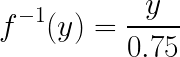
Now, let’s "reverse" the apple buying question: if you spent $2.25 on apples, how many pounds did you buy? The answer is 2.25 / 0.75 = 3, so you bought three pounds. This kind of "reversal" of a function is called the function's inverse. In the example without the intercept, the inverse is:
Note that in this notation, the "-1" indicates that you're taking the inverse of a function, not a reciprocal.
One thing to look out for is that the domain can change. For instance, suppose your original function is:
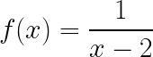
This function is defined for all real numbers except 2, since the denominator cannot be zero. The inverse of this function is
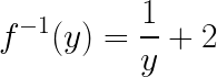
For the same reason, the inverse function is defined for all inputs except 0.
Another gotcha to pay attention to is that the resulting inverse might not be a function because of having multiple outputs for a single input. Consider the function y = x2. Its reverse would therefore be:
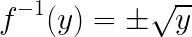
As you can see from the plus/minus, the inverse has two outputs for one input, so it is not a function unless we restrict the domain (for example, to x ≥ 0)
Graphically, a function and its inverse (if it exists) are mirror images across the line y=x. Consider the function y = x3. The graph of this function and its inverse is: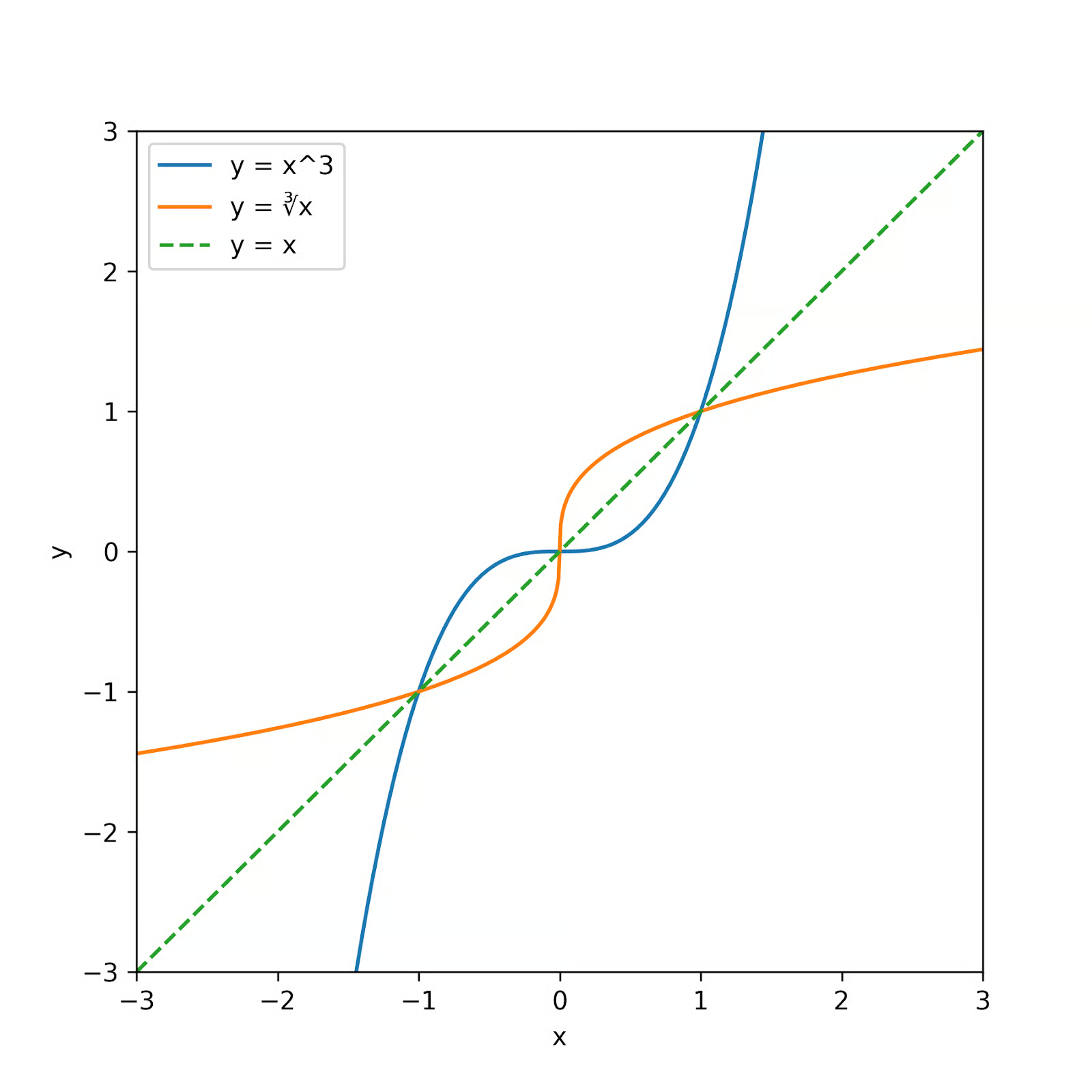
The original function (in blue) has an inverse (in orange) which is reflected across the line y = x.
Let’s look at two types of functions that are closely related: exponential and logarithmic functions.
Suppose you deposit $100 in a savings account that pays 10% interest, compounded annually.
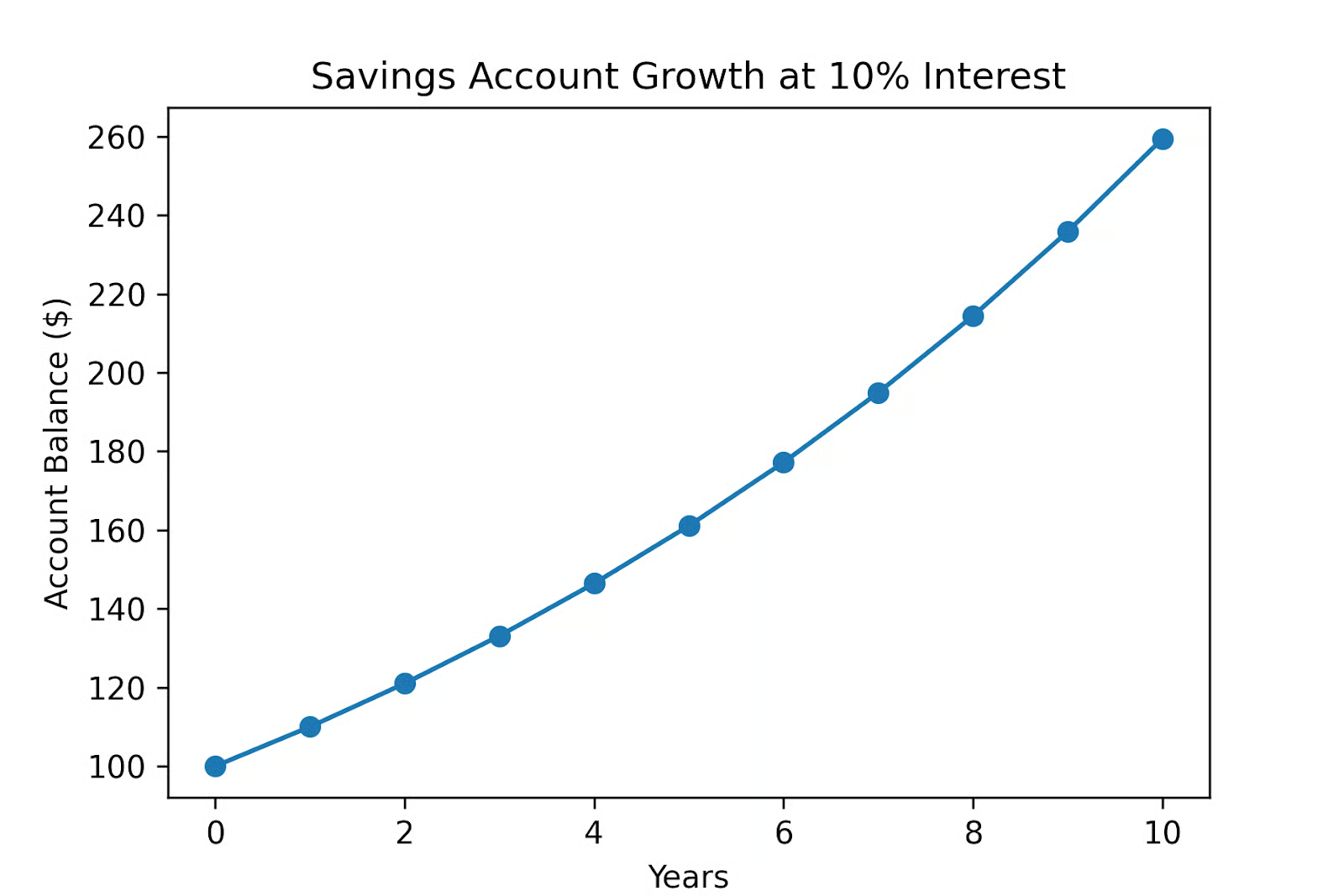
This is an example of exponential growth. Each step multiplies the previous step by a fixed amount. The general function for exponential growth is y = A bx, where y is the output, x is the input (often time), A is the initial amount, and b is the growth factor per unit of x.
In data science, exponential models show up in compound growth processes such as user growth or revenue growth, in probability models, and many other applications.
Logarithmic functions turn this question around. Now, instead of asking for the amount after x time has passed, suppose you want to know how long you need to let your money grow to reach $200, if you assume a compounding factor of 10%.
Now we need to know how many times 1.10 is multiplied by itself to get 2. This is the question logarithms answer.
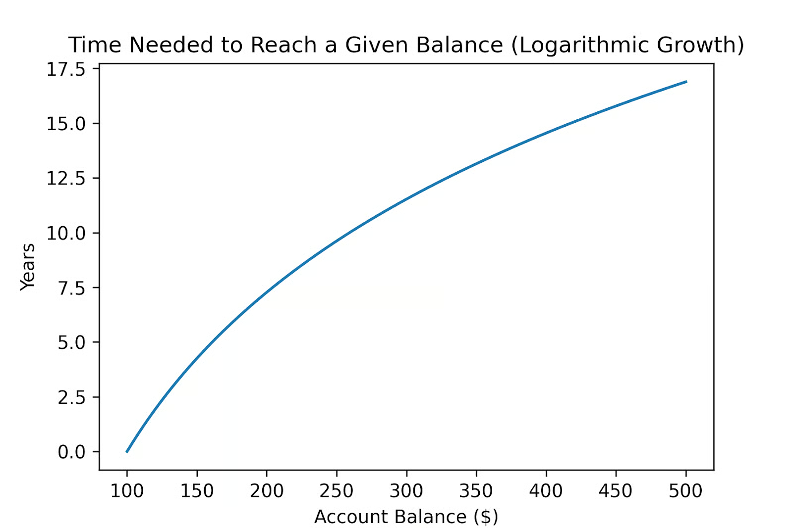
Looking at the graph, we see it will take a bit more than 7 years for our money to double.
As we worked out, logarithmic functions are the inverse of exponential functions. Exponential models ask questions like: after x months, what is the growth rate? Logarithmic models ask: given a growth rate, how many months did it take to get there?
Data scientists often use logarithms to make a skewed distribution manageable. For instance, income distributions are usually extremely right-skewed: a few high earners stretch the top of the distribution, while most people are clustered at the low end.
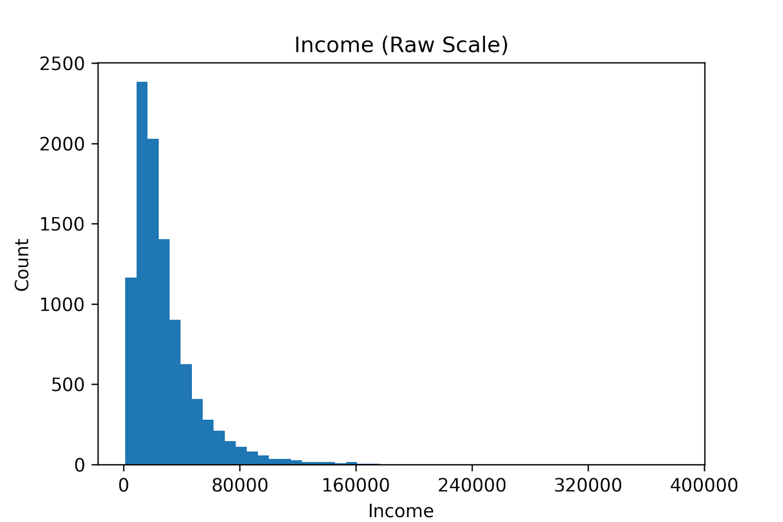
You can transform the data by taking the logarithm of each data point:
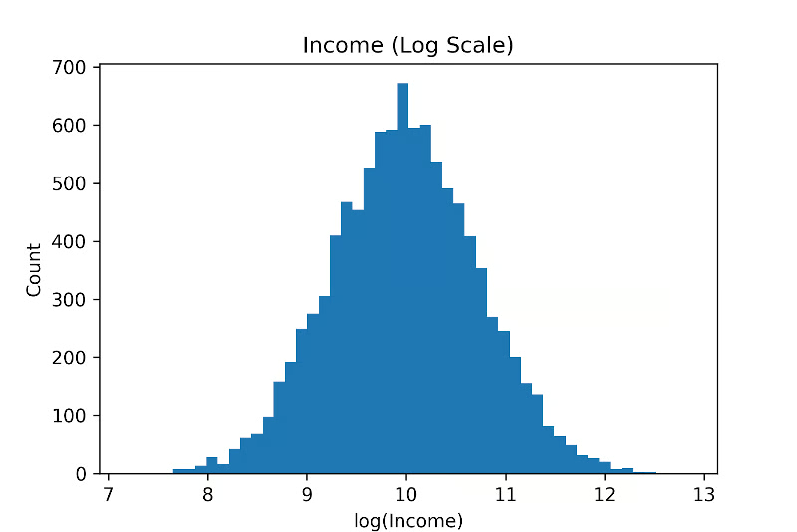
Large incomes are compressed while other incomes are spread out. Log transforms change the question from absolute differences to relative differences. As a result, the long right tail collapses, and the distribution often becomes roughly normal. Now, the variance is more stable, and we can apply linear regression.
The logarithm plays a central role in one of the most commonly used loss functions in binary classification, which is known as Cross-Entropy Loss or log loss, defined for a single sample as:

Here, the binary variable y (0 or 1) is the true value for a sample, and p is the predicted probability that y is class 1.
Log loss strongly penalizes confident but incorrect predictions. Predicting a probability close to 0 when the true label is 1 (or vice versa) results in a large penalty, while uncertain predictions incur smaller penalties. This makes log loss well-suited for training probabilistic classifiers such as Logistic Regression.
Activation functions are used in neural networks to ensure the output of each layer is nonlinear. Common activation functions are sigmoid and ReLU functions.
The Sigmoid Function is a smooth, S-Shaped function that is defined by the following formula:

It takes any real number as input and outputs a value strictly between 0 and 1. It is used to convert raw scores into probabilities.
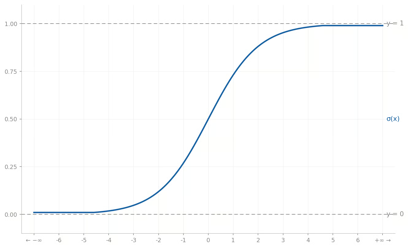
A common use case of the sigmoid function is in logistic regression for binary classification. Logistic regression computes a linear combination of the inputs to produce a score. That score is then converted into a probability using the sigmoid function. Probabilities above a threshold (typically 0.5) are classified as 1, and those below the threshold are classified as 0.
For more on that matter, refer to our Python Logistic Regression and Logistic Regression in R tutorials.
The Rectified Linear Unit (ReLU) function converts negative numbers to 0 and leaves positive numbers unchanged. It is defined as:

For values over 0, it’s the same as the identical function, as you can see from its graph:
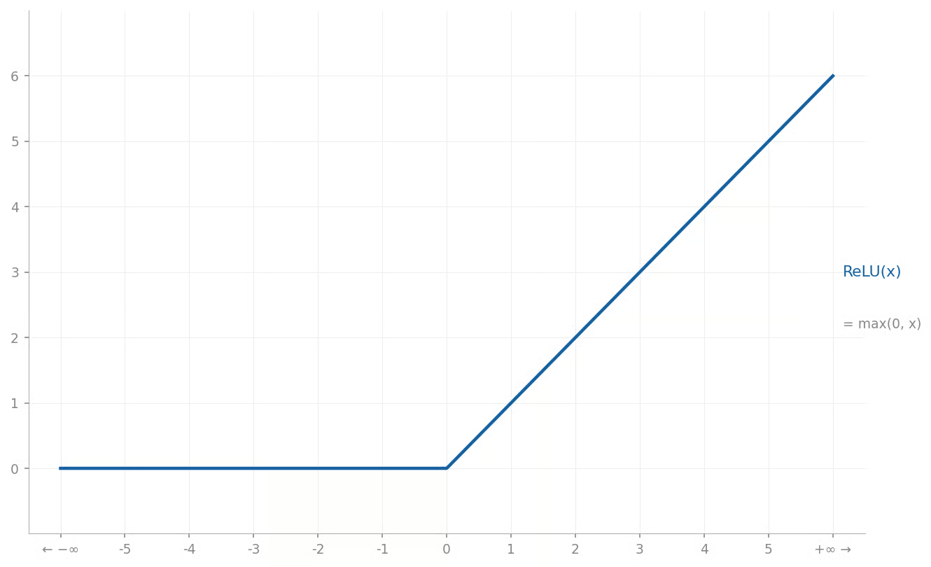
Like the sigmoid function, it acts as a nonlinear activation function in the hidden layers of a Neural Network. However, it is computationally simple, requiring only a maximum operation, whereas the sigmoid requires an expensive exponential function call.
Because a ReLU sets all negative values to 0, it produces sparsity in the network, where many neurons are zeroed out. This can reduce noise and lead to more efficient representations.
Another shape of non-linear functions can be found in decision trees, which recursively partition the input space into smaller regions by splitting on features and thresholds until a stopping criterion is met.
Each resulting leaf node is assigned a prediction value. Thus, a decision tree can be viewed as a piecewise function, where each region of the domain maps to a constant prediction value. By stitching together many local rules, decision trees can capture complex patterns.
For instance, you might see a two-dimensional region partitioned as follows:
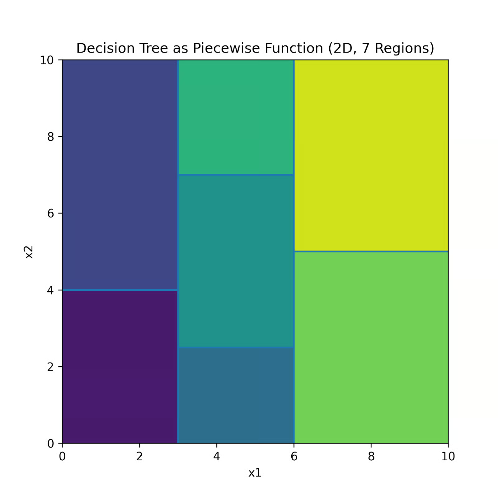
This heat map corresponds to the following regions:
|
Region |
Domain piece |
Function value |
|
1 |
x1 < 3 and x2 < 4 |
1 |
|
2 |
x1 < 3 and x2 >= 4 |
2 |
|
3 |
3 ≤ x1 < 6 and x2 < 2.5 |
3 |
|
4 |
3 ≤ x1 < 6 and 2.5 ≤ x2 < 7 |
4 |
|
5 |
3 ≤ x1 < 6 and x2 ≥ 7 |
5 |
|
6 |
x1 ≥ 6 and x2 < 5 |
6 |
|
7 |
x1 ≥ 6 and x2 ≥ 5 |
7 |
Function optimization is the process of finding input values that maximize or minimize a function. For instance, you might want to maximize a profit function or minimize an error function. The study of function optimization is known as "operations research" and is a huge and ongoing body of mathematical theory.
Optimizing functions is closely connected to a function’s local and global "extrema" (maximum or minimum points). A "local minimum" is a minimum within a particular range, and a "global minimum" is the minimum of the function overall.
For example, consider the function f(x) = x4 - 3x2 + x.
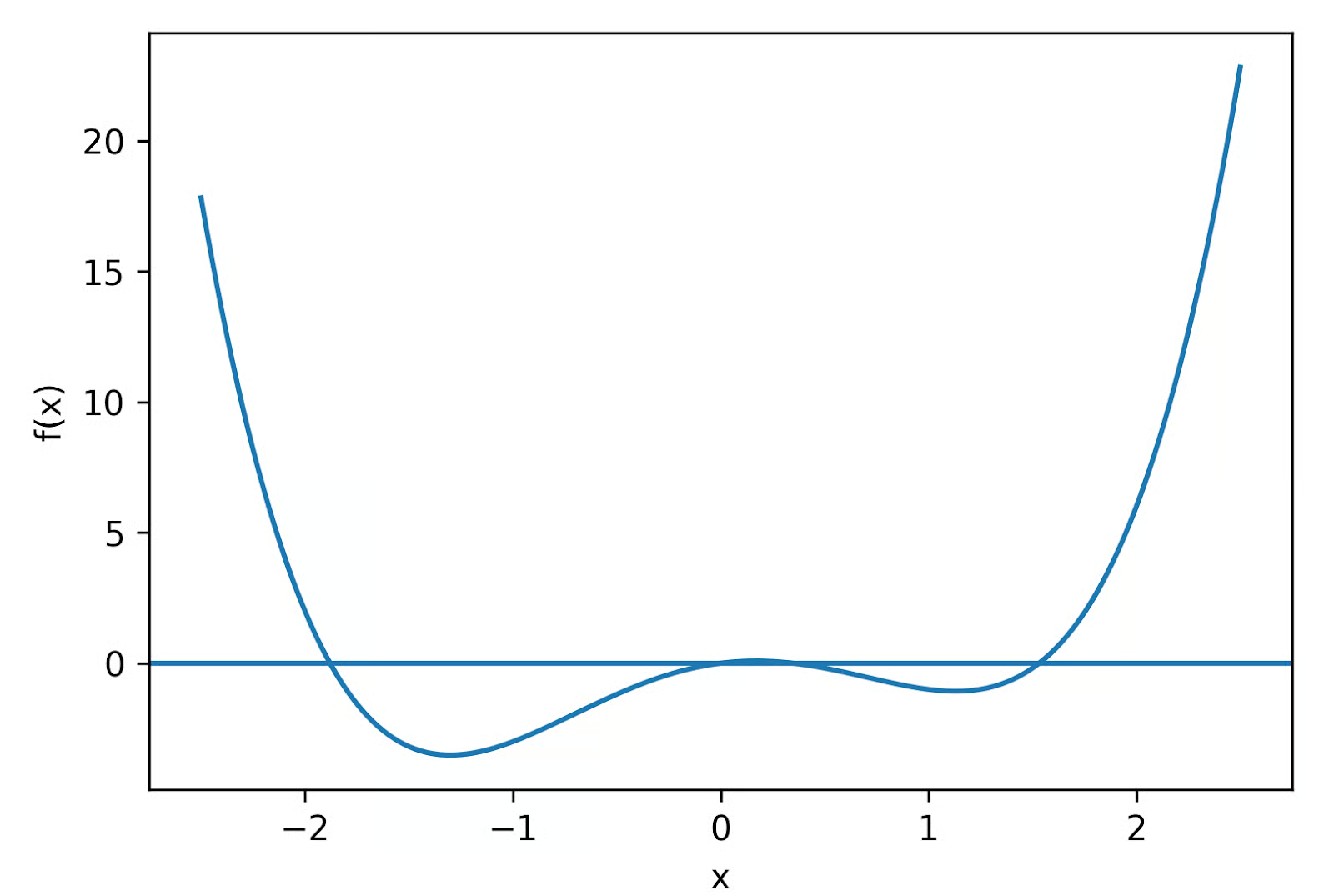
There are two local minima: one when x is approximately -1.30 and another when x is approximately 1.13. The y value is lower when x is -1.30, so that is the function's global minimum.
For simple optimization tasks like finding the best price to maximize profit in a one‑variable pricing model, it is sufficient to take the derivative of the function, set it to zero, and solve for x. For training deep neural networks, it is not as simple as that, but it works in a similar way.
The most important optimization method for Deep Learning is Gradient Descent. The gradient is the multi‑dimensional generalization of the slope, telling us how the loss changes with respect to each parameter.
It works by repeatedly moving in the direction of the steepest downhill change of a function. At each step, it uses the gradient to decide which way to move and a step size to decide how far. Over time, this process leads toward a local minimum.
Functions are ubiquitous in mathematics, programming, and data science. "Learning" in machine learning really is just finding the best function (and its parameters) to map inputs to outputs. Now that you know about functions, code some up in Python or your favorite programming language!
To see how these ideas fit into real machine learning workflows, you can continue with the Understanding Machine Learning course.
Mathematical Courses
Cursus
Cursus
Cursus
blog
Zoumana Keita
14 min
blog
DataCamp Team
11 min
Tutorial
Iheb Gafsi
Tutorial
Mark Pedigo
Tutorial
Javier Canales Luna
Tutorial
Richmond Alake
