
Track
Quantitative Analyst in R
67 hr
Cost functions act as the "scorekeeper" of decisions. They measure how far predictions deviate from actual values of a dataset versus predicted values. In machine learning, they guide optimization algorithms to minimize error and improve model accuracy.
In this article, we build intuition step by step. We start with economic applications, where cost functions describe the trade-off between production and efficiency. We then turn to machine learning, where they drive model training. Next, we examine optimization as the bridge between the two. Finally, we explore real-world examples.
Cost functions are fundamental to optimization and evaluation. Let's define cost functions mathematically and examine their key properties.
A cost function (also called an "error function") maps one or more input variables into a single numeric value that represents the "cost" of a decision or prediction. In machine learning, it is usually defined as the average of the loss function over all samples in the dataset.
The cost function plays two roles: it serves as an objective an optimization algorithm minimizes, and as an evaluation metric to measure how well a model performs.
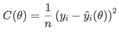
Let's look at a cost function as an objective. For each house, the loss function penalizes the difference of the actual sale price and the predicted price. The cost function aggregates these penalties across all houses:
A smaller cost indicates a better overall fit, while a larger cost indicates a greater average error. The optimizer adjusts the parameters to minimize this cost.
As an evaluation metric, cost functions measure performance. For instance, a classifier might be evaluated with accuracy, or recall, or whichever metric is appropriate for the application. In this way, cost functions provide a way to judge success.
Three mathematical properties are especially relevant.
Together, these properties determine how tractable a cost function is for optimization. When one of these properties is missing, special techniques may be required to compensate.
Cost functions describe the relationship between the quantity of output and the total cost of products. They are an essential tool to understand firm behavior, pricing strategies, and profit analysis.

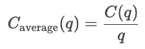
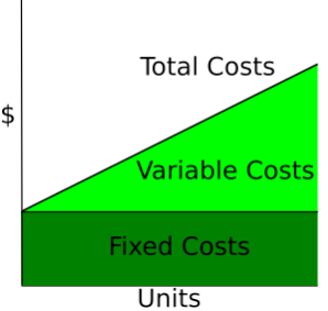
Cost curves show how costs vary as a function of total quantity produced. Fixed costs are constant, so are displayed as a horizontal line, while variable costs rise as a function of the units produced.
Wikipedia: Cost Curve
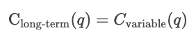
In the short run, at least one input, such as capital or plant size, is held constant, and other inputs vary. Short-run costs measure how efficiently a firm operates with its current setup. So, for a given quantity q, the cost in the short term is the sum of the fixed costs and the variable costs dependent on quantity.
![]()
In the short-run, optimize within the current capacity.
In the long run, all inputs are variable. The firm might scale its production processes. Long-run costs measure efficiency when capacity itself can change, showing the minimum achievable cost for any output level
In the long run, optimize by choosing the optimal capacity itself.
Cost functions are used to analyze pricing behavior. Firms compare cost curves with market prices to help decide whether to expand or contract production. If the marginal cost is below the market price, producing more increases profit; if the marginal cost is less than the market price, producing more units costs money.
Cost functions are also used in pricing strategies. They determine the minimum viable price a firm can charge. Firms may change above the marginal cost to maximize profit, or closer to the MC in highly competitive industries. Thus, cost analysis informs break-even pricing, cost-plus pricing, and dynamic pricing strategies.
The break-even point occurs where total revenue equals the total cost.![]()
At this point, the company covers all costs but makes no profit. Producing fewer results in a loss, whereas producing more generates profit.
Profit is the difference between total revenue and total cost.
![]()
If marginal revenue exceeds marginal cost (MR > MC), the firm will increase output to generate more profit. If marginal revenue is less than marginal cost (MR < MC), the firm will decrease output to gain additional profit. The firm maximizes profit by producing the quantity where MR = MC.
For more information about finance, I recommend checking out these DataCamp resources.
In ML applications, cost functions quantify the residuals (the difference between predicted values and actual values) over the entire dataset. This section explores the main families of cost functions and how they shape model behavior.
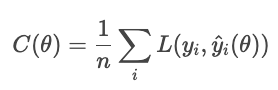
In a machine learning context, the goal of regression (not necessarily linear regression) is to predict a continuous value. A regression loss function quantifies the error between actual and predicted values for a particular sample; cost functions aggregate loss functions into an overall quantity. Optimization processes use cost functions to minimize the overall error.
We focus on the four main families of cost functions: mean absolute error (MAE), mean squared error (MSE), root mean square error (RMSE), and Huber loss.
Different cost functions handle errors differently. In effect, they define how severely to punish deviations between predicted and actual values. The MAE applies a uniform penalty, representing median behavior and robustness to outliers. The MSE squares each residual, causing large errors to dominate and punishing them more severely. The Huber loss blends these two, using a quadratic penalty for small errors and a linear one for large ones (beyond a threshold δ).
The mean absolute error is defined as the average of the absolute value of the residuals.
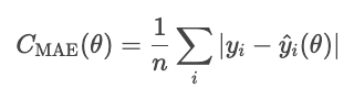
The MAE treats all deviations equally, so it is not as affected by outliers as other methods we'll see, such as the MSE. However, the absolute error is awkward mathematically and makes gradient-based optimization more difficult.
A note about the function parameter. θ represents the model parameters. The optimizer controls cost based on these parameters, not directly on the predicted values that arise from them. Therefore, we write the cost as a function of the θ, not Ŷi.
The mean squared error (MSE) is given by the following formula.
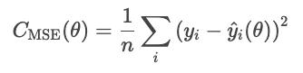
Squaring residuals exaggerates large errors, which makes MSE sensitive to outliers. However, this form of error is differentiable and convex, which makes it friendly for optimization.
A drawback of the MSE is that its units are squared. For instance, in a housing prices regression model, the loss is in dollars squared, which lacks intuitive meaning. The RMSE corrects this issue by taking the square root of the MSE.
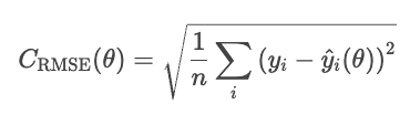
RMSE behaves similarly to MSE but the units are in the same units as the problem (dollars, not squared dollars).
The Huber loss is less sensitive to outliers in the data than the MSE (or RMSE). It combines MAE and MSE, and controls the transition with a parameter δ.
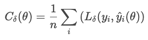
where
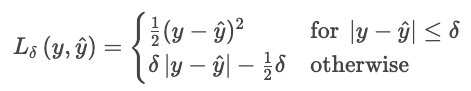
This formula prevents a few large residuals from dominating the loss. The Huber loss is a good choice for noisy real-world data where you expect occasional extreme observations.
Classification predicts discrete categories. These cost functions compare probability distributions against true labels, penalizing incorrect or overconfident predictions.
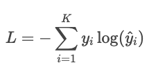
Cross-entropy loss (log loss) rewards a model when it is confidently correct and punishes it when it is confidently wrong.
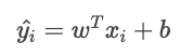
For a classifier that outputs pure probabilities Ŷ, the likelihood of the observed label Y is
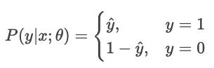
Maximum-likelihood estimation (MLE) maximizes this likelihood over all samples.
Let's turn this idea into minimizing cost. Minimizing is the same as maximizing the negative, so let's flip the sign. Let's also take logs.
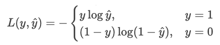
We can write this more succinctly as a single sum.
![]()
Why the log? The log has several advantages
Suppose a model predicts probabilities for two choices: "dog" (choice 0) or "cat" (choice 1). If the real answer is 1 ("cat") and the model is 90% certain it is a cat, the loss is small because the model was confident and correct. If the model says it's 10% certain it's a cat, the loss is large, because the model was confident but wrong.
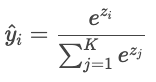
When there are more than two classes ("cat", "dog", "bird"), the model produces a raw score ("logit") for each class, denoted Zi. Logits can be any real number, so they are converted into probabilities that sum to one via the softmax function.
The model's predictions are then compared with the actual labels using the cross-entropy.
Example
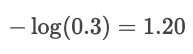
Suppose the true label is "cat" and the model predicts probabilities: cat: 80%, dog: 15%, bird: 5%. The loss is
![]()
If the predicted probability for "cat" were only 30%, then the loss would be much higher:
The log punishes confident mistakes and rewards high-confidence predictions.
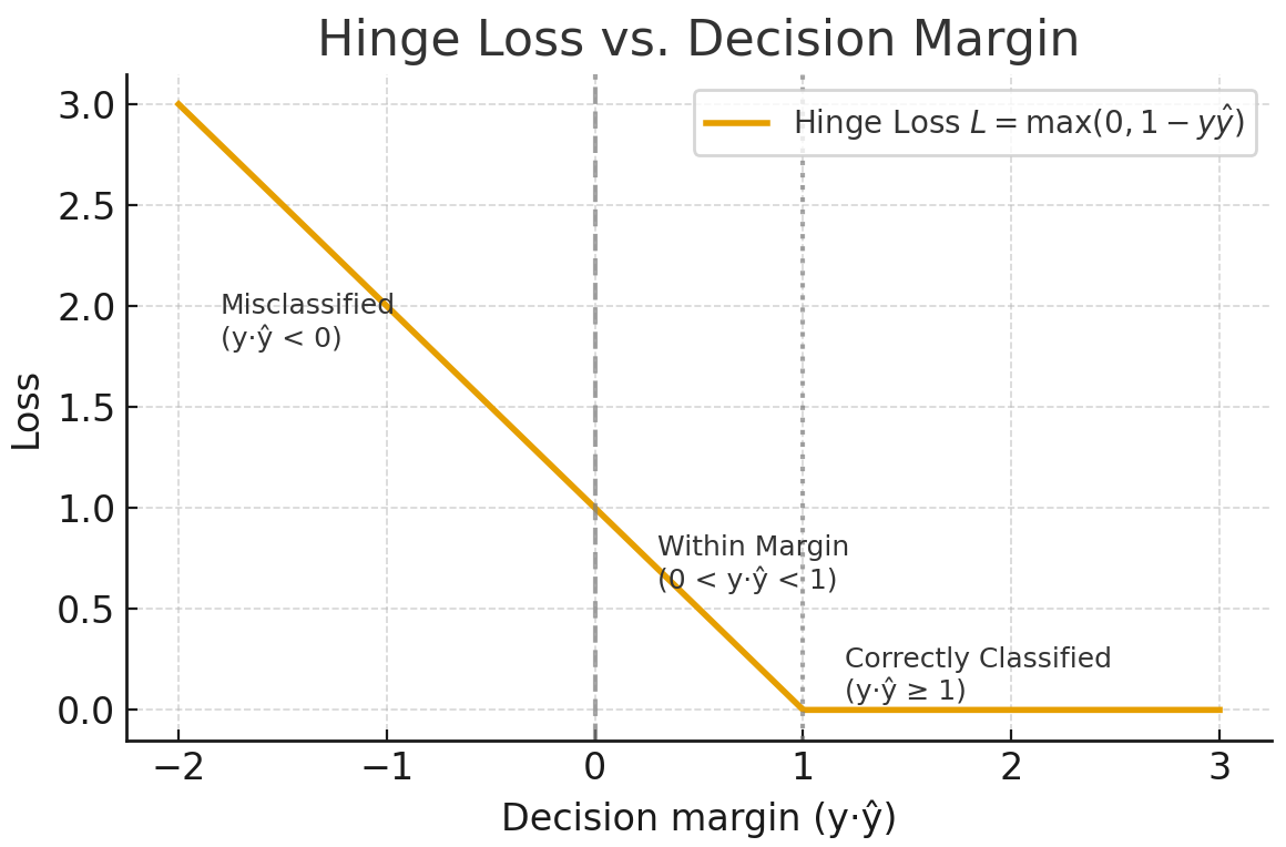
The hinge loss is mostly used for max-margin classification, as in support vector machines (SVMs). The goal is to classify confidently by keeping predictions far from the decision boundary.
For binary classification, the hinge loss is given by the following formula.
![]()
where
The total cost function is
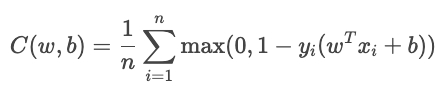
The term YiŶi measures how well the sample is classified.
Generated by ChatGPT 5
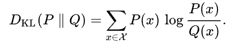
The Kullback-Leibler (KL) divergence is a measure of how much an approximating probability distribution Q differs from a given probability distribution P. It is defined as
Wikipedia
The KL divergence can be interpreted as the average difference of the number of bits for encoding samples of P using a code optimized for Q.
Regularization techniques prevent models from fitting noise in the training data by adding a term to the cost function that penalizes overly complex solutions.
Without regularization, the model minimizes the loss:
With regularization, the model adds a penalty term
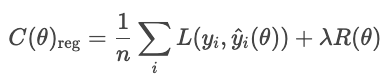
where
Common types of regularization are L1, L2, and elastic net.
L1 regularization (aka lasso) adds the absolute value of each model weight to the cost function.
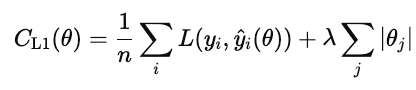
When this cost is minimized, many weights get driven to zero. This makes L1 a form of automatic feature selection. Features that don't contribute get pushed to zero.
L2 regularization (aka ridge regression) penalizes the square of each model weight.
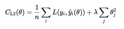
Unlike L1 it does not set weights exactly to zero, but shrinks them smoothly. This keeps all the features in the model but reduces their influence to stabilize predictions.
Elastic net adds both L1 and L2.
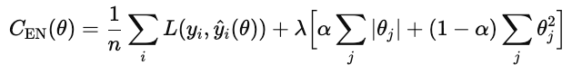
λ controls how strong the overall regularization is. α is a number between 0 and 1 that control the percentages of L1 versus L2, where 1 is pure L1 and 0 is pure ridge.
The different classification loss strategies have trade-offs.
Cross-entropy maximizes the correct probability by penalizing confident wrong answers. Trade-offs are that it is sensitive to outliers and mislabeled data. It works best when you care about confidence quality (e.g., risk models).
Hinge loss enforces a margin so that correct classifications aren't just correct, but confidently correct. It ignores values samples that are safely beyond the margin and gives a linear penalty for violations. It is less sensitive to outliers than cross-entropy, but more difficult to optimize smoothly, as it is not differentiable at the hinge.
Kullback-Leibler(KL) divergence matches one probability distribution to another. It is equivalent to cross-entropy minus the entropy of the true distribution.
For more information, check out these links.
So far, we've discussed cost functions in theory. In practice, the success of an ML model depends on how efficiently it minimizes those functions. In this section, we introduce practical details of core optimization algorithms and tuning strategies.
Optimization is the process of finding the optimal values of model parameters that minimize a cost function. In ML, this means discovering the parameters that make predictions as close as possible to actuals.
Gradient descent is the standard algorithm for optimizing cost functions. It iteratively updates model parameters in the direction that most reduces the cost, the negative gradient. Conceptually, it measures the multi-variable slope of the cost function and steps downhill.
The update rule is
![]()
where θ are the model parameters, n is the learning rate, and ![]() is the gradient of the cost function with respect to the parameters.
is the gradient of the cost function with respect to the parameters.
The choice of learning rate is critical. If it is too large, updates overshoot the minimum and oscillate or diverge. If it's too small, convergence becomes slow and may stall in local minima.
The main variants are batch, stochastic, and mini-batch.
Standard gradient descent applies a fixed learning rate to all parameters. In complex models, different parameters may need different step sizes. Adaptive optimizers adjust learning rates based on the history of gradient magnitudes.
![]()
Each parameter's learning is scaled inversely to this average. This prevents oscillation and allows stable progress even when some parameters have steep gradients. RMSProp is widely used for recurrent networks and noisy data.
![]()
It converges fast, is robust to noisy data, and is the default optimizer for deep network frameworks.
Before optimizing with gradient descent, scale features so that they operate on comparable ranges. Proper scaling improves the stability and efficiency of optimization.
Without scaling, features with large numeric ranges dominate the gradient. Gradient descent then zigzags instead of taking direct steps toward the minimum.
There are two common approaches.
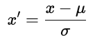
where u is the mean and ơ is the standard deviation. Standardization preserves the structure of the data.
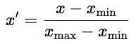
Normalization is common in neural networks, where activation functions perform best with bounded inputs.
Parameter initialization strongly influences model training. Poor initialization can cause slow convergence, exploding or vanishing gradients, or models that fail to learn. Good initialization places parameters in a region of the cost surface where gradients are stable.
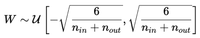
This keeps activations and gradients roughly constant across layers.
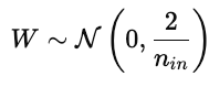
This prevents gradients from vanishing too quickly during backpropagation.
A training loss curve plots the model's error on the training dataset over time. It shows how well the model updates its parameters to minimize the error. A steadily decreasing curve indicates the model is learning patterns from the data.
The validation loss curve shows the model's ability to generalize on unseen data, such as a hold-out or validation set. It indicates the model's ability to predict on previously unseen data.
Ideally, both curves decrease at the beginning of the curve, then flattens. This demonstrates that the model is both learning effectively and generalizing effectively.
Overfitting occurs when the model learns noise as if it were signal, and doesn't generalize well. This appears in a graph showing training and validation curves when the training loss decreases but the validation loss increases. Fixes include using a larger dataset, or employing regularization in the model.
Underfitting occurs when the model fails to capture the underlying patterns in the data. Both training and validation curves remain high. In this case, try more data, a more complex model, or reduce regularization.
Convergence is the point where the curve flattens out, and ore training offers little improvement. This is the sweet spot between overfitting and underfitting.
We have seen how economics and machine learning rely on optimization to guide decision-making and training. Both fields endeavor to make the best decisions based on a metric of cost or loss. Let's delve into optimization theory more generally.
An objective function is a mathematical function that defines what we want to minimize or maximize. In the cases we've seen so far, we've minimized cost or error. For econ, we looked at cost curves, and with ML, we looked at regression losses (MAE, RMSE, Huber), and classification losses (cross-entropy, hinge loss, KL loss). These are both examples of optimizing an objective function.
Often, we want to optimize multiple, often conflicting, goals. A company might want to maximize profit while minimizing risk. A data scientist might want to improve model accuracy without sacrificing interpretability or fairness. Such competing goals define a multi-objective optimization problem in which improving one objective might worsen another.
A solution is Pareto optimal if no objective can be improved without making at least one other objective worse. The set of Pareto-optimal solutions forms the Pareto frontier, a curve that consists of the best achievable trade-offs. Each point on this curve represents a different balance of priorities.
For example, increasing a model's complexity might improve accuracy but reduce interpretability. Simpler models are easier to explain but may perform worse. The Pareto frontier includes the "best trade-offs" and excludes solutions that are dominated by other variables.
Choosing the right point depends on context and judgment. You might assign weights to each goal or use policy restraints.
When outcomes are uncertain, optimization minimizes expected loss, the average loss over all possible scenarios. In ML, this idea appears in the risk function.
![]()
where L(Y,f(x)) is the loss for a given prediction, and the expectation averages over the data distribution. The goal is to find the model f that minimizes this expected loss. This model performs best on average, not just on individual samples.
The Bayes risk is the theoretical lower bound of expected loss. Formally, it is given by the following formula.
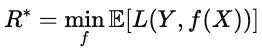
Intuitively, it is the "perfect score", i.e., the smallest achievable value under perfect information about the data distribution. The closer a model's performance is to Bayes risk, the more optimal it is.
Cost functions are used in any industry that makes data-driven decisions. They help balance competing objectives and formalize what "better" means. These functions balance competing objectives and guide optimization. The same logic used to train ML models is used to optimize real-world processes.
In manufacturing, for instance, cost functions quantify losses, such as inventory loss. An inventory cost function balances the expense of excess stock against penalties for shortages. Similar frameworks are used for production scheduling or energy use to minimize expected total cost under uncertainty.
In healthcare, predictive models use cost functions to balance accuracy and resource allocation. For instance, a readmission risk model identifies high-risk patients early so that clinicians can intervene with follow-up calls or home visits. Missing a high-risk patient is more costly than flagging a low-risk one, so the function penalizes those errors differently.
Finance also uses objective functions. For example, credit scoring models predict the probability that a borrower will default on a loan within a set period of time, say twelve months. Approving a risky borrower results in potential financial loss, while rejecting a safe borrower potentially loses revenue. The model minimizes expected cost.
Across all these domains, cost functions balance trade-offs into measurable quantities that decision makers can use and reason with.
Cost functions provide a method for evaluating decisions. In economics, they model the trade-off between output and efficiency. In machine learning, they measure the gap between predictions and truth.
In ML, cost functions are the foundation of model design. The choice of loss functions determines what the model considers "success." Mean squared error rewards overall accuracy, cross-entropy rewards calibrated probabilities, and hinge loss rewards confident separation.
Across all domains and industries, the underlying logic works the same: define an objective and optimize it. Cost functions translate vague goals into concrete numbers that guide optimization.
Cost functions are useful in economics, machine learning, manufacturing, finance, healthcare, and everywhere else one might want to quantify trade-offs.
For more information, I recommend these DataCamp resources.
Top DataCamp Courses
Track
Course
Course
blog
Zoumana Keita
14 min
Tutorial
Richmond Alake
Tutorial
Mark Pedigo
Tutorial
Mark Pedigo
Tutorial
Mark Pedigo
Tutorial
Mark Pedigo
