
Course
Intermediate Python
4 hr
1.4M
Imagine you're trying to map the quickest route through a maze, identify connections between people in a social network, or find the most efficient way to transmit data across the internet. These challenges share a common goal: to systematically explore relationships between different points. Breadth-first search is an algorithm that can help you do just that.
Breadth-first search is applied to a wide range of problems in data science, from graph traversal to pathfinding. It is particularly useful for finding the shortest path in unweighted graphs. Keep reading and I will cover breadth-first search in detail and show an implementation in Python. If, as we get started, you want more help in Python, enroll in our very comprehensive Introduction to Python course.
Breadth-first search (BFS) is a graph traversal algorithm that explores a graph or tree level by level. Starting from a specified source node, BFS visits all its immediate neighbors before moving on to the next level of nodes. This ensures that nodes at the same depth are processed before going deeper. Because of this, BFS is useful for problems that require examining all possible paths in a structured, systematic way.
BFS is useful for finding the shortest path between nodes, because the first time BFS reaches a node, it uses the shortest route. This makes BFS useful for problems like network routing, where the goal is to find the most efficient route between two points. The diagram below shows a simplified explanation of how BFS explores a tree.

Breadth-first search is designed to explore a graph or tree by visiting all neighbors of a node before progressing to the next layer. This structured traversal ensures that all nodes at a particular depth are explored before moving deeper into the structure. This level-by-level approach makes BFS a systematic and reliable way to navigate complex networks.
BFS explores each node at the current depth level before moving on to the next. This means that all nodes at a given distance from the starting point are processed before moving deeper.
BFS uses a queue to manage nodes that need to be visited. The algorithm processes a node, adds its unvisited neighbors to the queue, and continues this pattern. The queue operates in a first-in, first-out manner, ensuring that nodes are explored in the order they are discovered.
In unweighted graphs, or graphs where every link is the same length, BFS guarantees finding the shortest path between nodes. Because BFS explores neighbors level by level, the first time it reaches a node, it does so via the shortest possible route. This makes BFS especially effective for solving shortest-path problems, in situations where all edges have equal weight.
BFS works with both graphs and trees. A graph is a network of connected nodes that may have cycles, like a social network, while a tree is a hierarchy with one root and no cycles, like a pedigree. BFS is useful for both, making it broadly applicable to a wide range of tasks.
Let’s demonstrate the breadth-first search algorithm on a tree in Python. If you need to refresh your Python skills, check out the Python Programming skill track at DataCamp. For more information on different data structures and the algorithms, take our Data Structures and Algorithms in Python course and read our Data Structures: A Comprehensive Guide With Python Examples tutorial.
Let's get started. First, we need to set up a simple decision tree for our BFS to search.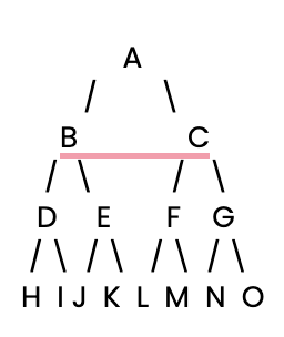
Next, we’ll define this simple decision tree using a Python dictionary, where each key is a node, and its value is a list of the node's children.
# Define the decision tree as a dictionary
tree = {
    'A': ['B', 'C'],  # Node A connects to B and C
    'B': ['D', 'E'],  # Node B connects to D and E
    'C': ['F', 'G'],  # Node C connects to F and G
    'D': ['H', 'I'],  # Node D connects to H and I
    'E': ['J', 'K'],  # Node E connects to J and K
    'F': ['L', 'M'],  # Node F connects to L and M
    'G': ['N', 'O'],  # Node G connects to N and O
    'H': [], 'I': [], 'J': [], 'K': [],  # Leaf nodes have no children
    'L': [], 'M': [], 'N': [], 'O': []   # Leaf nodes have no children
}
Now let’s implement the BFS algorithm in Python. BFS works by visiting all nodes at the current level before moving to the next level. We’ll use a queue to manage which nodes to visit next.
from collections import deque  # Import deque for efficient queue operations

# Define the BFS function
def bfs(tree, start):
    visited = []  # List to keep track of visited nodes
    queue = deque([start])  # Initialize the queue with the starting node

    while queue:  # While there are still nodes to process
        node = queue.popleft()  # Dequeue a node from the front of the queue

        if node not in visited:  # Check if the node has been visited
            visited.append(node)  # Mark the node as visited
            print(node, end=" ")  # Output the visited node

            # Enqueue all unvisited neighbors (children) of the current node
            for neighbor in tree[node]:
                if neighbor not in visited:
                    queue.append(neighbor)  # Add unvisited neighbors to the queue
Now that we’ve created our BFS function, we can run it on the tree, starting at the root node A.
# Execute BFS starting from node 'A'
bfs(tree, 'A')
When we run this, it outputs each node in the order it was visited.
A B C D E F G H I J K L M N OThe traversal pattern of BFS is straightforward in trees, since they are inherently acyclic. The algorithm starts at the root and visits all children before moving to the next level. This level-order traversal mirrors the hierarchical relationships in trees: each node has one parent and multiple children, leading to a predictable pattern.
In contrast, graphs can contain cycles. Multiple paths between nodes can lead back to previously visited nodes. This can be a problem for BFS, requiring careful management of revisits. Keeping track of which nodes have been visited prevents unnecessary reprocessing and helps avoid cycles that could cause loops. In our earlier BFS implementation, we used a visited list to ensure each node was processed only once. If a visited node was encountered, it was skipped, allowing BFS to continue smoothly.
How efficient is breadth-first search? We can use Big O notation to evaluate how the efficiency of BFS changes as a function of graph size.
The time complexity of BFS is O(V+E), where V is the number of vertices (nodes) and E is the number of edges in the graph. This means BFS’s performance depends on both the number of nodes and the connections between them.
The space complexity of BFS is O(V) due to the memory needed to store nodes in the queue. In wider graphs, this may mean storing many nodes at once. At the worst case, it may mean holding every node at once.
Breadth-first search has numerous practical applications in fields like computer science, networking, and artificial intelligence. Its methodical level-by-level exploration makes it ideal for searching and pathfinding problems.
One application of BFS is in network routing algorithms. When data packets traverse a network, routers use BFS to find the shortest path. By exploring all neighboring nodes before moving deeper, BFS quickly identifies efficient routes, minimizing latency and enhancing performance.
BFS is also useful for solving puzzles, like mazes or slider puzzles. Each position is a node, and connections are edges. BFS can efficiently find the shortest path from the start to the exit.
Another powerful use is in social network analysis. BFS helps discover relationships between users and identify influential nodes. It can explore social connections and discover clusters of related users, revealing insights into network structures.
BFS is useful in AI training as well. For example, it can be used for searching game states in games like chess. AI algorithms can use BFS to explore possible moves level by level, evaluating future states to determine the best action, thus finding the shortest path to victory.
BFS is also applied to robotics for path planning. It enables robots to navigate complex environments by mapping surroundings and finding paths while avoiding obstacles.
Let’s compare BFS to other common search algorithms, like depth-first search and Dijkstra’s algorithm.
Breadth-first search and depth-first search (DFS) are both graph traversal algorithms, but they explore graphs differently. BFS visits all neighbors at the current depth before moving deeper, while DFS explores as far down one path as possible before backtracking.
BFS is great for finding the shortest path in unweighted graphs. This advantage makes it good for problems like maze navigation and networking. In contrast, DFS may not always find the shortest path, but it can be more space-efficient in deep, wide graphs. This makes it preferable for tasks such as topological sorting or scheduling problems, where a complete traversal is needed without excessive memory use.
Dijkstra’s algorithm is a graph traversal algorithm designed for weighted graphs, where edges have varying costs. Unlike BFS, which treats all edges equally, Dijkstra calculates the shortest path based on edge weights. It’s most useful for applications where cost matters, such as finding the optimal route while considering travel time.
While Dijkstra is powerful for weighted graphs, it is more complex and computationally intensive. Dijkstra has a time complexity of O((V+E)logV) when using priority queues, which is significantly higher than BFS’s time complexity O(V+E). You can learn more about Dijkstra’s Algorithm in Implementing the Dijkstra Algorithm in Python: A Step-by-Step Tutorial.
One problem you may encounter when using BFS is getting caught in a cycle. A cycle occurs when a path returns to a previously visited node, creating a loop in the traversal. If BFS does not track visited nodes properly, this can lead to an infinite loop. It’s important to maintain a list of visited nodes or mark each node as explored once processed. This simple approach should ensure your BFS explores the graph efficiently and terminates properly.
Another common pitfall is incorrect queue usage. BFS depends on a queue to keep track of which nodes need to be explored. If the queue isn’t managed properly, it can result in missing nodes or incorrect paths in the traversal. To avoid this, add nodes to the queue in the order they need to be explored and then remove them. This helps BFS explores nodes level by level, as intended. Using a reliable data structure, like collections.deque in Python, helps.
Despite its versatility, BFS is not be the best choice in every situation. For one thing, BFS is not always suitable for very large or deep graphs, where depth-first search may be more practical. Also, BFS is not appropriate for weighted graphs, because BFS treats all edges equally. Algorithms like Dijkstra’s or A* are better suited for these cases, as they account for varying costs when calculating the shortest path.
BFS is particularly valuable for finding the shortest path in unweighted graphs. Its level-wise exploration makes it an excellent tool for situations that require a thorough exploration of nodes at each depth level.
If you’re interested in search algorithms, be sure to check out my other articles in this series, including: Binary Search in Python: A Complete Guide for Efficient Searching. You may also be interested in AVL Tree: Complete Guide With Python Implementation, and Introduction to Network Analysis in Python.
Learn Python with DataCamp
Course
Course
Course
Tutorial
Amberle McKee
Tutorial
Rajesh Kumar
Tutorial
Amberle McKee
Tutorial
Amberle McKee
Tutorial
Benito Martin
Tutorial
Bex Tuychiev