Step by Random Step: Exploring the Random Walk Model

In my first coding-based statistics course in college, my teacher proposed a question: how can we model the Brownian motion of a single pollen particle in a dish of water? After several misguided attempts, my classmates and I eventually stumbled on the correct answer: a random walk. I later learned that this simple model is used to model all sorts of things, from animal movements to stock price fluctuations.

In this article, we’ll explore the mathematical foundations of random walks, examine different types, and discuss their applications. Part of what makes the random walk interesting is that it is used in so many different disciplines. In addition to my example, in physics, it helps describe particle movement; in finance, it models stock price fluctuations; and in biology, it explains animal movement patterns. Random walks capture real-world randomness, which is key for simulating stochastic processes.

For those looking to build a strong foundation in the statistics that underpin random walk theory, we recommend starting with the Introduction to Statistics in R course or the Introduction to Statistics in Python course.

What Are Random Walks?

In probability theory, a random walk is a model describing a sequence of random steps that make up a path. Or else, we could say that a random walk is a mathematical model that describes a path formed by a sequence of steps, each determined independently and with a certain probability. This stochasticity makes random walks inherently unpredictable.

Imagine a person taking a step in a random direction at each moment. Over time, their path forms an unpredictable, meandering trail. Despite its simplicity, this concept has surprising depth and versatility, modeling various real-world scenarios that involve randomness.

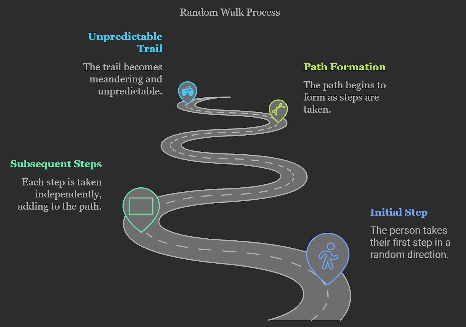
A conceptual explanation of a random walk. Image courtesy of napkin.ai.

The idea of random walks dates back to early probability studies. One of the earliest examples, often called the drunkard’s walk, illustrates how a person stepping randomly will wander erratically rather than move predictably toward a destination. This randomness, combined with the assumption that each step is independent of previous ones, laid the foundation for modern random walk models.

Understanding the Mathematics of Random Walks

To understand random walks, let’s start with a simple case: a one-dimensional (1D) random walk. Imagine a particle on a number line. It’s able to move either +1 or -1 along the number line with each step. Each move is determined by an equal probability of stepping right or left. Over time, the particle's position forms a probability distribution that spreads out, representing the likelihood of finding it at various locations.

This principle can be expanded to two or three dimensions. In a two-dimensional (2D) random walk, the particle moves on a plane and can step in any of the four cardinal directions (up, down, left, right) with equal probability. Similarly, in a three-dimensional (3D) random walk, the particle moves in space and can step in any of the six possible directions (up, down, left, right, forward, backward) with equal probability. These higher-dimensional random walks capture even more complex and realistic scenarios.

A defining feature of random walks is their stochastic nature, meaning each step depends only on the current position and not on the previous steps. This makes them a type of Markov process—a mathematical concept where the future state depends solely on the present state, not on the sequence of events that preceded it. This "memoryless" movement, combined with probability distributions describing potential positions, provides a solid mathematical foundation for understanding random walks.

We can analyze a random walk using statistical properties to understand its behavior over time. This involves examining aspects like the expected distance from the starting point, the probability distribution of possible positions, and the likelihood of returning to the origin. These analyses help us quantify randomness and predictability, provide insights into patterns, and make predictions.

Key Properties of Random Walks

Random walks have several important properties that help us understand their behavior and applications. Here are some key aspects to consider:

Expectation and variance

In a one-dimensional random walk, we can calculate the expected distance (or mean position) from the starting point over time. If each step has an equal probability of moving left or right, the expected position after many steps remains zero, implying that, on average, the walker stays near the starting point.

However, the variance of the position, which measures the spread or dispersion of possible positions, increases with each step. Specifically, in a symmetric random walk, the variance grows linearly with the number of steps, making it a useful indicator of the typical distance from the origin over time.

Autocorrelation

While simple random walks have no correlation between steps (each step is independent of the last), certain types of random walks introduce autocorrelation, where past steps can influence future ones. For example, in a biased random walk, steps may have a slight tendency in one direction, causing positions to be more predictable.

Autocorrelation in a random walk impacts how we model and predict the walk’s progression. This is especially relevant in applications where past behavior influences future steps, such as certain financial models.

Central limit theorem

The central limit theorem (CLT) tells use that the sum of a large number of independent random variables tends to follow a normal (or Gaussian) distribution, regardless of the original distribution. In the context of random walks, this means that as the number of steps increases, the distribution of positions tends to resemble a normal distribution. This is a useful property because it allows us to approximate the probability of finding the walker at certain distances from the starting point.

Law of large numbers

The law of large numbers (LLN) explains that as the number of trials or steps increases, the average of the results converges to the true average. For random walks, this means that while the average position remains zero, the variance and range of possible positions grow predictably with each additional step. This principle helps bridge the gap between pure randomness and predictable statistical patterns in large samples.

Types of Random Walks

Random walks vary widely depending on the rules governing each step. These types influence how the walk behaves. Some are designed for simple or structured environments while others are equipped for more complex, real-world phenomena. Let’s explore some of the most common types of random walks.

1D, 2D, and 3D random walks

The dimensionality of a random walk plays a fundamental role in its behavior. In a 1D random walk, each step is either a move forward or a move backward along a line. This makes the walk relatively easy to model and predict.

However, as we move to 2D (plane) and 3D (space) walks, the possible paths increase significantly, introducing new behavior. For instance, in a 2D random walk, the probability of returning to the starting point remains high, while in a 3D random walk, this probability decreases.

This change is important in fields like physics and chemistry, where particles might diffuse differently depending on the dimensional constraints.

Lattice random walk

In a lattice random walk, movement is confined to discrete points on a grid or lattice. This type of walk is commonly used in physics and network theory, where nodes are arranged in a grid, and movement can only occur to neighboring nodes.

A common example is a 2D lattice, where each step allows movement to adjacent points on a Cartesian grid. This constraint simplifies modeling by limiting movement paths, which is useful when simulating complex networks or molecular structures.

Gaussian random walk

In a Gaussian random walk, each step's size is determined by a Gaussian (or normal) distribution. Instead of moving by a fixed distance, the step size varies according to a bell-curve distribution, with most steps being small and occasional larger jumps. This type of walk is frequently used in financial modeling to account for the variability in asset price changes.

Heterogeneous and biased random walks

Heterogeneous and biased random walks allow for variation in step direction and size based on certain probabilities. This flexibility makes them more adaptable to real-world scenarios.

In a heterogeneous random walk, the probability of moving in any direction might change based on location or external conditions. For example, animals foraging for food may favor areas with known resources, creating a biased random walk. These walks are useful for studying behaviors that depend on contextual factors.

Random walk with drift

In a random walk with drift, there is a consistent tendency to move in one direction. For instance, stock prices may exhibit an overall upward trend over time despite daily fluctuations. The drift in these walks represents an external force or trend influencing the path. This type is often seen in finance, where models incorporate a drift term to represent growth or decline, providing a more realistic approach to predicting asset prices and market trends.

Each of these types of random walk serves a unique purpose, offering different ways to model random, yet structured, behavior. The dimensional constraints, distribution of steps, and presence of drift or bias make random walks highly versatile for data modeling and simulation across fields.

Real-World Applications of Random Walks

Random walks are more than just theoretical constructs; they play an essential role in many practical applications across disciplines. Let’s explore how random walks inform real-world problem-solving across sectors.

Applications in data science and machine learning

Computer science

Random walks underpin several computer science algorithms, such as random sampling, web graph traversal, and image segmentation. For example, Google’s PageRank algorithm used random walks to rank web pages based on their relevance, simulating how a user might randomly navigate between links on the internet.

Feature extraction

In machine learning, random walks can help extract features by highlighting relationships within data points. For example, in network analysis, random walks can reveal clusters or communities, assisting in tasks like recommendation systems and social network analysis.

Anomaly detection

Random walks can also be used to detect anomalies in datasets. For example, if data points deviate significantly from a typical path in a random walk model, these points might indicate unusual events or errors in the data. Anomaly detection is especially valuable in fields like cybersecurity and fraud detection.

Simulating stochastic processes

Random walks simulate stochastic, or randomly determined, processes, allowing data scientists to model unpredictable real-world phenomena. By simulating random walks, we can gain insights into systems where precise prediction is challenging, such as weather patterns or customer behavior.

Time series forecasting

In time-series analysis, random walks form the basis for certain forecasting models, including the random walk hypothesis in finance. These models assume that future values in a time series depend solely on the most recent value, with no correlation to past trends. For more on time series forecasting, check out ARIMA for Time Series Forecasting: A Complete Guide. Also, take our Forecasting in R course with Professor Hyndman, who connects random walk models to naive and seasonal naive forecasting methods.

Applications in other fields

Finance

One of the most notable uses of random walks is in financial modeling, especially for predicting stock prices. The efficient market hypothesis suggests that stock price movements are essentially random, as new information is instantly absorbed, making future prices unpredictable. Random walks can be used to model stock price changes over time, illustrating how prices fluctuate without a predictable path.

Mathematics

In pure mathematics, random walks provide solutions to complex problems. For instance, they are useful in solving Laplace’s equation, analyzing networks, and exploring combinatorics.

Physics and chemistry

In the physical sciences, random walks are crucial for modeling diffusion processes, such as the way molecules spread through a medium. Brownian motion, where particles suspended in a fluid move unpredictably due to collisions with surrounding molecules, is a classic example that can be accurately simulated using random walks. This is actually how I first learned about random walks.

Biology

Random walks are valuable in ecology for studying animal movement patterns. Animals foraging for resources may seem to move in a random walk, sometimes biased toward regions with known resources. Other biological concepts, such as the spread of populations or genes, can often be modeled with random walk principles, making it easier to understand and predict changes within ecosystems.

Special Cases and Variants of Random Walks

In addition to the classic random walk, several advanced variants extend the concept to fit specialized applications.

Self-avoiding walks

A self-avoiding walk is a random walk in which the path does not revisit any position it has already passed. This variant is particularly useful in fields like polymer chemistry, where it can model how polymer chains form without crossing themselves. Because each step avoids previously visited points, self-avoiding walks are more constrained than traditional random walks. This means they’re computationally challenging but useful for understanding non-overlapping paths in confined spaces.

Branching

In branching random walks, the path can split into multiple branches, with each branch following a random walk. This type of walk is instrumental in modeling branching processes such as cell division or the spread of information through networks. Each "branch" represents an independent random path that originates from a common source.

Correlated walks

Correlated walks take this concept a step further, where each step's direction is partially influenced by the previous step. This variant is useful for modeling inertia in systems where changes happen gradually rather than randomly. Correlated walks are often applied in finance to simulate price trends or in movement ecology to understand how animals navigate their environments with some memory of their past direction.

Loop-erased walks

A loop-erased walk is a variant where loops, or paths that cross themselves, are removed as they form. Each time a step revisits a position, the intervening loop is erased, leaving a streamlined, non-repeating path. Loop-erased walks are commonly applied in network analysis and maze generation algorithms because they create paths that avoid redundancy.

Implementing Random Walks in Python

Let’s try implementing a random walk in Python. To get started, ensure you have Python installed (we’ll use Python 3.10) and the necessary libraries available. You can install any missing libraries using pip. Here’s what we’ll use:

import numpy as np # for numerical operations and generating random steps
import matplotlib.pyplot as plt # for plotting and visualizing the random walks

1D random walk

We’ll start with a simple one-dimensional random walk, where each step is either +1 or -1, chosen randomly.

# Parameters
n_steps = 100  # Number of steps

# Generate random steps: +1 or -1
steps = np.random.choice([-1, 1], size=n_steps)

# Calculate positions
positions = np.cumsum(steps)

# Plot the random walk
plt.figure(figsize=(10, 6))
plt.plot(positions, marker='o', linestyle='-', markersize=4)
plt.title("1D Random Walk")
plt.xlabel("Step")
plt.ylabel("Position")
plt.grid(True)
plt.show()

This generates a simple random walk and visualizes the progression over time. Here’s the ouput when I run this code:

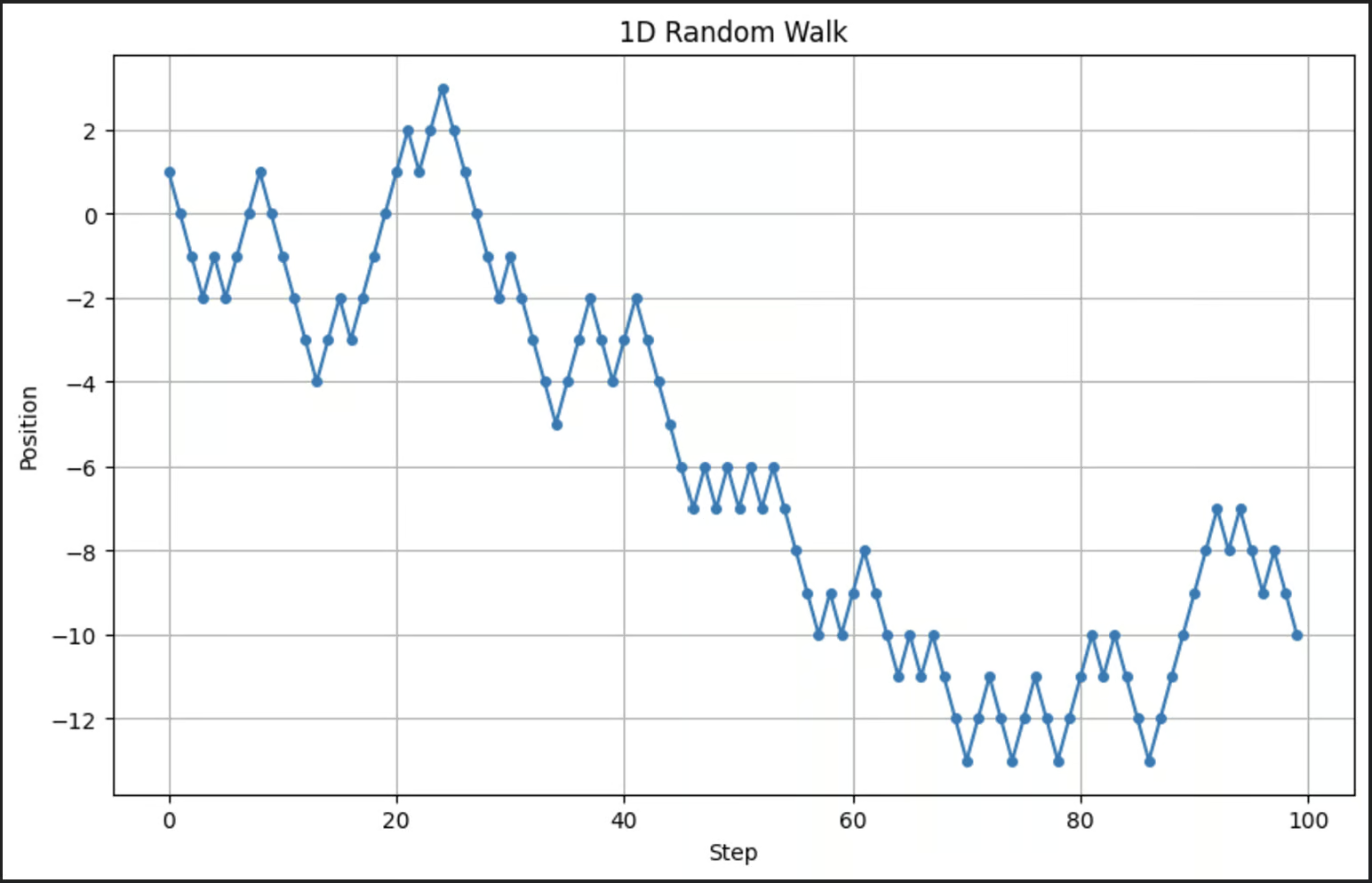
Now remember, we’re running a stochastic model. This means that every time we run it, the output will look a little different.

2D random walk

Now let’s extend the random walk to two dimensions. At each step, the direction will be chosen randomly.

# Parameters
n_steps = 500

# Generate random steps in x and y directions
x_steps = np.random.choice([-1, 1], size=n_steps)
y_steps = np.random.choice([-1, 1], size=n_steps)

# Calculate positions
x_positions = np.cumsum(x_steps)
y_positions = np.cumsum(y_steps)

# Plot the 2D random walk
plt.figure(figsize=(8, 8))
plt.plot(x_positions, y_positions, marker='o', linestyle='-', markersize=2, label='Random Walk')
plt.plot(x_positions[0], y_positions[0], 'ro', markersize=8, label='Start')  # Red dot for start
plt.plot(x_positions[-1], y_positions[-1], 'ko', markersize=8, label='End')  # Black dot for end
plt.title("2D Random Walk")
plt.xlabel("X Position")
plt.ylabel("Y Position")
plt.grid(True)
plt.axis('equal')  # Ensures equal scaling for both axes
plt.legend()
plt.show()

This code creates a visually engaging path in two dimensions.

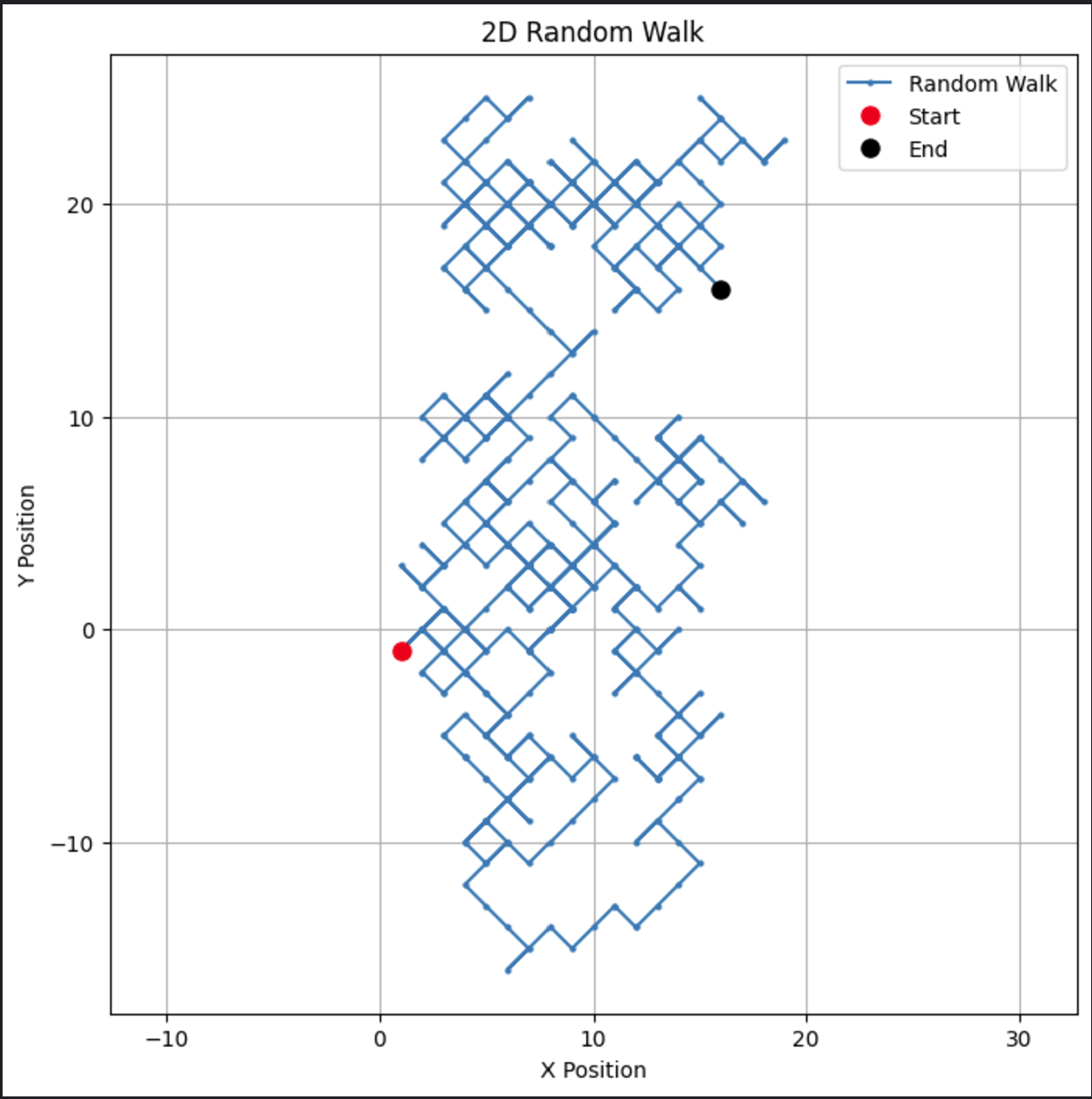
This type of two-dimensional random walk could be modified to accommodate applications like particle motion or spatial modeling.

Biased random walk

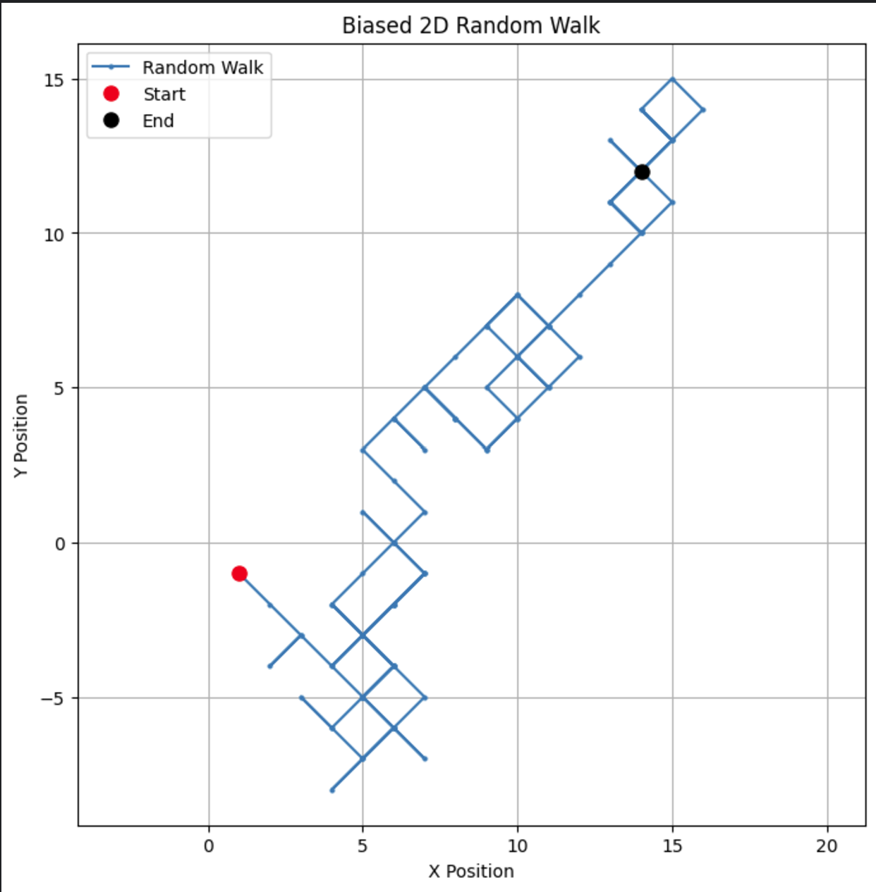
Lastly, let’s look at a slightly more complex example: a biased random walk. To introduce bias, we can adjust the probabilities of each step direction. For example, we might make upward steps more likely.

# Parameters
n_steps = 100
bias = 0.7  # Probability of stepping +1

# Generate biased random steps in x and y directions
x_steps = np.random.choice([-1, 1], size=n_steps, p=[1-bias, bias])
y_steps = np.random.choice([-1, 1], size=n_steps, p=[1-bias, bias])

# Calculate positions
x_positions = np.cumsum(x_steps)
y_positions = np.cumsum(y_steps)

# Plot the biased 2D random walk
plt.figure(figsize=(8, 8))
plt.plot(x_positions, y_positions, marker='o', linestyle='-', markersize=2, label='Random Walk')
plt.plot(x_positions[0], y_positions[0], 'ro', markersize=8, label='Start')  # Red dot for start
plt.plot(x_positions[-1], y_positions[-1], 'ko', markersize=8, label='End')  # Black dot for end
plt.title("Biased 2D Random Walk")
plt.xlabel("X Position")
plt.ylabel("Y Position")
plt.grid(True)
plt.axis('equal')  # Ensures equal scaling for both axes
plt.legend()
plt.show()

By changing the bias, you can observe how the walk tends to favor a particular direction, simulating real-world scenarios like drift in stock prices or animal migration patterns.

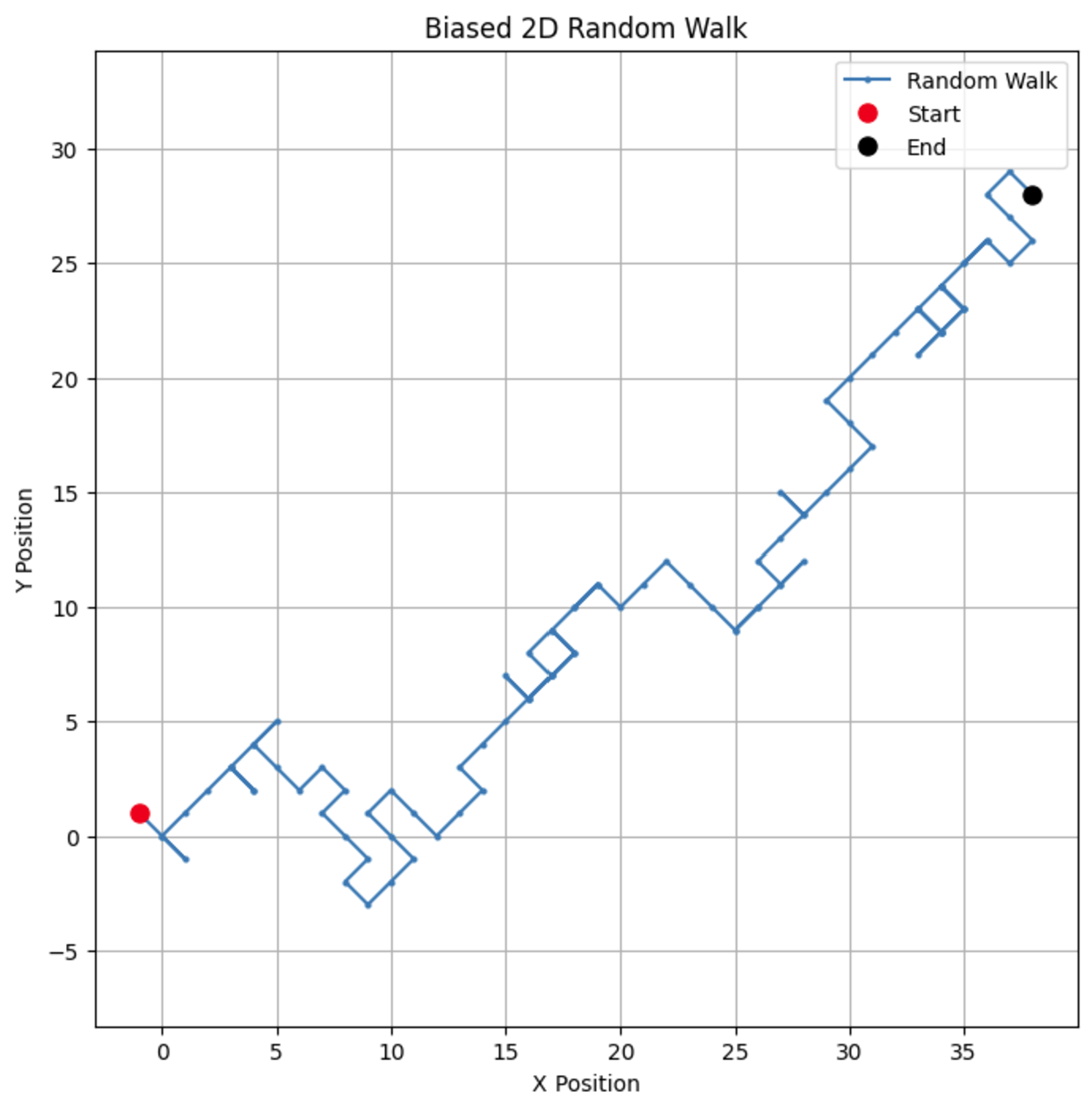
If we change the bias parameter to 0.55, we can see a dramatic difference in the way the model behaves. While it still has a bias for going up, the bias is not as strong, leading to more loops and detours.

Conclusion

Random walks are a valuable modeling tool for data scientists, applicable in fields from physics to finance and beyond. Their ability to model complex, stochastic processes makes them indispensable in many real-world scenarios.

Hungry for more? Check out DataCamp’s suite of probability and statistics courses. You’ll find all sorts of great courses in both Python and R. If you’re interested in more advanced content, check out DataCamp's course on Statistical Simulation in Python and the Introduction to Machine Learning tutorial. Or if you’re ready to test your knowledge, tackle some of these probability puzzles.