A Comprehensive Guide to Using ANOVA in Excel

Statistical analysis is fundamental to data-driven decision-making in various fields, including business, healthcare, education, and scientific research. One commonly used statistical method in academic and business settings is the Analysis of Variance, or ANOVA.

Microsoft Excel provides a powerful and user-friendly platform for conducting ANOVA. Its intuitive interface benefits beginners, eliminating the need for specialized statistical software like SPSS or SAS.

This guide will simplify the process of conducting ANOVA in Excel, providing clear, step-by-step instructions to help you confidently perform and interpret ANOVA tests. Whether you’re a student, a researcher, or a professional looking to enhance your analytical skills, this guide will help you learn how to leverage Excel for one of your common statistical needs.

What is ANOVA?

ANOVA is a statistical method used to determine if there are significant differences between the means of three or more independent groups. They are similar to another statistical test called the t-test, which is used to determine if there is a significant difference between the means of two groups. ANOVA and t-tests represent two of many statistical techniques covered in our comprehensive Data Analysis in Excel course, which is worth visiting if you are serious about becoming proficient in statistics.

ANOVA works by comparing the variance within each group to the variance between the groups to assess whether the means of the groups are equal. If the between-group variance is significantly larger than the within-group variance, it suggests that at least one group mean differs from the others.

Broadly speaking, there are two types of ANOVA:

• One-Way ANOVA: A one-way ANOVA examines the effect of a single independent variable on a dependent variable by comparing the means of three or more groups.
• Two-Way ANOVA: A two-way ANOVA evaluates the impact of two independent variables simultaneously and examines their interaction. 

Academic researchers use these tests to analyze the results after performing a controlled study. For example, researchers could use ANOVA to compare the efficacy of different treatments or drugs across multiple patient groups. For-profit cmpanies could use ANOVA to arrive at data-driven decisions, such as comparing customer satisfaction scores between several service centers, or the performance of advertisement campaigns.

Why Microsoft Excel Is Good for ANOVA

Here are the ordered steps required to perform ANOVA manually. For reference, the f-ratio is the test statistic used in ANOVA to determine if there are significant differences between the group means. It involves multiple calculations to arrive at the statistic. 

1. Calculate the Overall Mean: Find the mean of all the data points combined.
2. Calculate the Group Means: Determine the mean for each individual group.
3. Compute the Total Sum of Squares: Measure the total variation in the data by summing the squared differences between each data point and the overall mean.
4. Compute the Between-Groups Sum of Squares: Measure the variation between the group means and the overall mean.
5. Compute the Within-Groups Sum of Squares: Measure the variation within each group by summing the squared differences between each data point and its group mean.
6. Calculate the Between-Groups Mean Square: Divide the between-groups sum of squares by the degrees of freedom between groups.
7. Calculate the Within-Groups Mean Square: Divide the within-groups sum of squares by the degrees of freedom within groups, where the degrees of freedom within groups is the total number of observations minus the number of groups.
8. Compute the F-Ratio: Divide the between-groups mean square by the within-groups mean square to determine the f-ratio.

As you can see, calculating ANOVA manually is a bit involved. For this reason, software is the way to go, and Microsoft Excel stands out due to its wide usage in most businesses and academic settings. 

Keep in mind, also, that, generally speaking, the ANOVA calculations are part of larger analytics projects. In addition to the statistical power of Excel, the availability of other features, such as beatuiful visualizations in Excel, adds weight to the argument that Microsoft Excel is a great tool for ANOVA. 

How to Enable the Data Analysis ToolPak in Excel

Add-ins in Excel are supplemental programs or features that can be installed and integrated with Excel to enhance its functionality. The Data Analysis ToolPak is one such add-in that helps with most data analytics requirements.

The Data Analysis ToolPak add-in isn’t enabled by default; hence you’ll have to check if you can spot the Data Analysis icon in the top-right corner under the Data tab, as shown below.

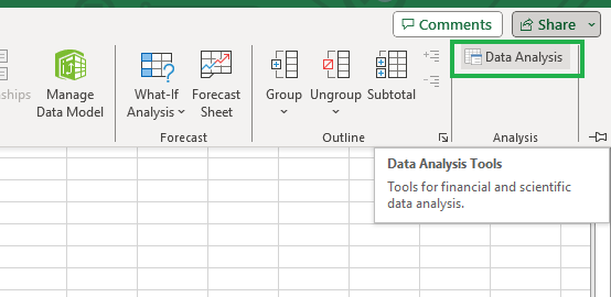
Data Analysis ToolPak in Excel

If you don’t see the Data Analysis ToolPak, it might mean it is not enabled. To enable it, click File from the menu and select Options.

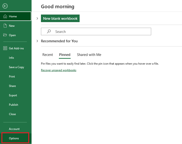Selecting Options from File Tab

Once the Excel Options dialog box has opened, select Add-ins.

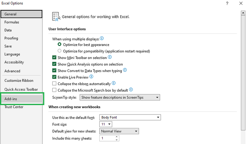Select Add-ins from the Excel Options dialog box

Next, in the Manage box at the bottom, select Excel Add-ins and click Go.

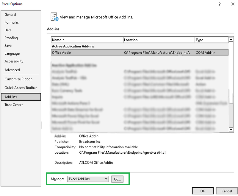Managing Excel add-ins

Under the Add-Ins box, check Data Analysis ToolPak and then click OK.

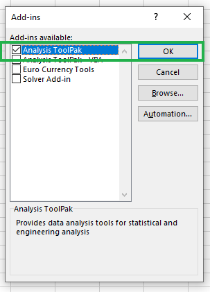
Enabling Data Analysis ToolPak

Now, when you check back in the Data Tab you will see the new Data Analysis icon. We are now ready to implement ANOVA in Excel using a few examples.

One-Way ANOVA in Excel: A Practical Example

Imagine you’re a data analyst in a marketing agency tasked with analyzing the performance of three marketing strategies (A, B, and C) on sales revenue.

Your company wants to determine if there is a significant difference in the mean sales revenue generated by these strategies. You have also collected sales revenue data from five different similar-scale companies in Region A, where each strategy was implemented.

The collected data has been tabulated in the table below:

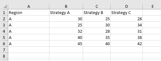
Data for one-way ANOVA

Let’s now use ANOVA to see if there is a significant difference between the mean sales of each strategy.

As the first step, select columns B, C, and D, including the first row as shown below, and click on the Data Analysis icon to open the Data Analysis Toolpak add-in.

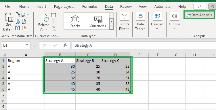Invoking the Data Analysis Toolpak add-in

Next, select Anova: Single Factor from the dialog box and click OK.

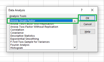
Selecting Anova: Single Factor option

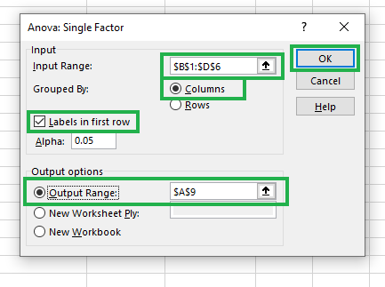
You will be prompted with a dialog box, as shown below.

Filling details for Anova: Single Factor

The Input Range is prefilled since we already selected it before invoking the add-in. Select Columns for the Grouped By option, check the Labels in the first row box, and leave the default values as they are. For the Output Range, we select a cell in the same sheet, say $A$9, or a new worksheet, as you wish.

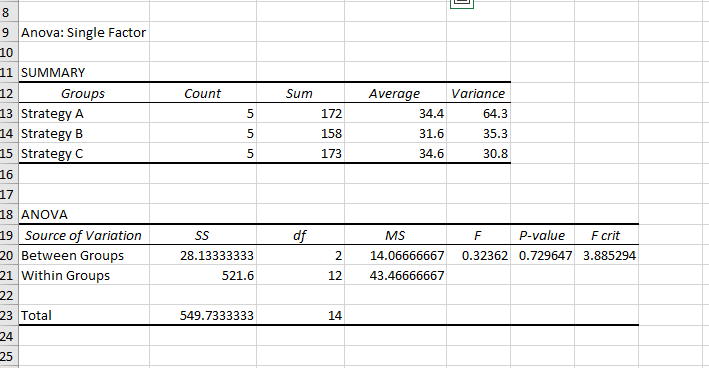
Click OK, and you will see the calculated results in the same Excel sheet.

One-way ANOVA results

You've successfully performed a One-way ANOVA on your dataset in no time!

Hypothesis testing and ANOVA

To better understand the results, we need to delve into hypothesis testing and its connection to ANOVA. Hypothesis testing is covered in detail in our Introduction to Statistics course.

In statistical hypothesis testing, the null hypothesis (H0) is a general statement asserting that there is no relationship between two measured phenomena. It posits no effect or no difference. The alternative hypothesis (H1 or Ha), on the other hand, suggests that sample observations are influenced by some non-random cause, contradicting the null hypothesis.

In our example, for a one-way ANOVA test, the hypotheses would be:

• Null Hypothesis (H0): There is no difference in the mean sales revenue generated by the three strategies.
• Alternative Hypothesis (Ha): At least one strategy has a different mean sales revenue.

The purpose of the ANOVA test is to test these hypotheses. If the p-value is less than the significance level (usually 0.05), we reject the null hypothesis in favor of the alternative hypothesis.

Interpreting the one-way ANOVA results

Reading the ANOVA table, we see three rows of results:

• Between Groups: This row represents the variation between the different marketing strategies and their related calculations.
• Within Groups: This row represents the variation within each marketing strategy and its related calculations.
• Total: This row represents the total variation in the data and the related results.

The P-value is 0.73. Since this is greater than the typical significance level of 0.05, we fail to reject the null hypothesis. In other words, there is not enough evidence to say that there is a significant difference between the means of the three marketing strategies.

The F crit value is 3.88. We know that if the f statistic (0.32) had been greater than the f-critical value, we would have rejected the null hypothesis and concluded that there is a significant difference between the means.

Based on our ANOVA test, it appears that the three marketing strategies do not significantly differ in their effectiveness. However, it’s important to remember that failing to reject the null hypothesis doesn’t prove that the null hypothesis is true. It just means that we don’t have strong enough evidence to conclude otherwise.

Let’s now find out how to test two factors and their influence on the dependent variable.

Two-Way ANOVA in Excel: A Practical Example

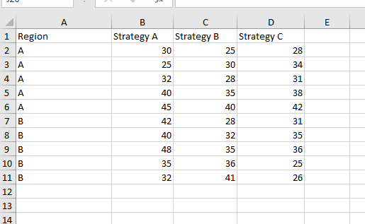
Let’s extend our earlier example to include a second factor. This time, your company wants to know if there are any significant differences in the revenue generated with different strategies, and also if there is an interaction effect between the strategies and regions.

The additional data collected has been added to the worksheet, as shown below:

Data for two-way ANOVA

Since there are now two factors - strategy and region - you know that we need a two-way ANOVA instead of a one-way ANOVA.

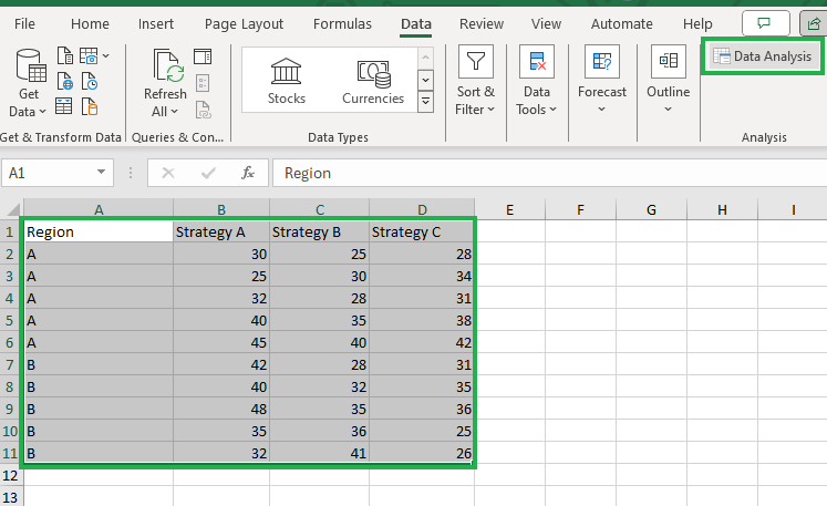
Let’s select the entire range of cells and click on the Data Analysis icon to invoke the add-in.

Invoking the Data Analysis Toolpak add-in

We’re presented with a dialog box with two different options for two-way ANOVA.

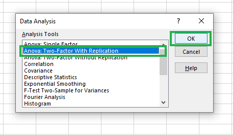
Selecting Anova: Two-Factor With Replication option

• ANOVA: Two-Factor With Replication: This is used when we have multiple observations, or replications, for each combination of our factors.
• ANOVA: Two-Factor Without Replication: This is used when we have only one observation for each combination of our factors.

In our case, since we have multiple observations for each combination of marketing strategy (A, B, C) and region (A, B), we choose a two-factor ANOVA with replication.

After clicking OK, you’ll see the dialog box below with a prefilled input range.

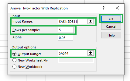
Filling details for Anova: Two-Factor With Replication

In the Rows per sample option, we input 5 because we have five data points for each of the regions. For the output range, we can select any cell, say $A$14, or a new worksheet as you wish. 

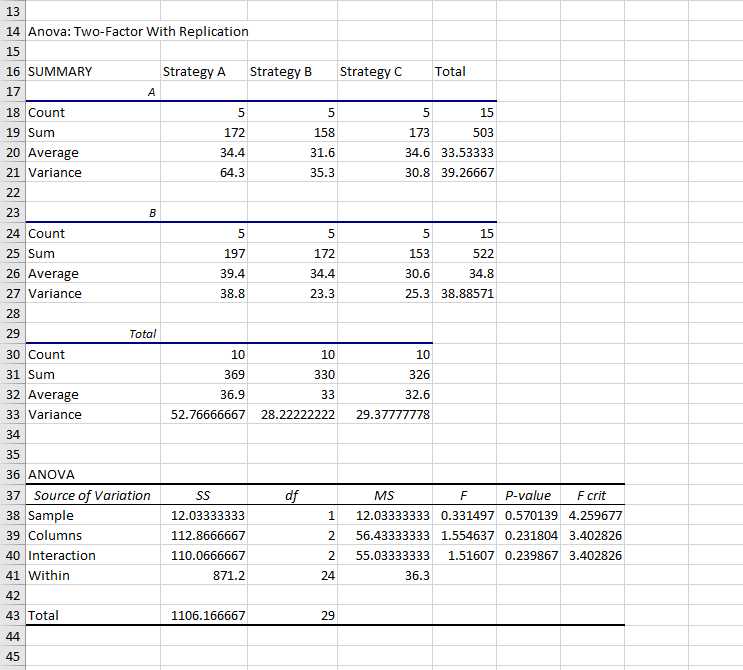Two-way ANOVA results

That’s it! You have performed Two-way ANOVA for the given dataset in a few steps.

Interpreting the two-way ANOVA results

Let's take a moment to understand how to read the ANOVA table and identify which row represents each factor tested.

• Sample: The Sample row represents the variation between the two regions.

• Columns: The Columns row represents the variation between the different marketing strategies.

• Interaction: The Interaction row represents the interaction effect between the marketing strategies and the regions.

• Within: The Within row represents the variation within each combination of marketing strategy and region.

• Total: The Total row represents the total variation in the data.

If the F statistic is sufficiently large, the p-value will be sufficiently small. This will lead us to reject the null hypothesis and conclude that there are significant differences between the means of the groups.

However, in our case, the f statistics for the sample, columns, and interaction are smaller than the f critical value for each, and the p-values are all larger than 0.05. Therefore, we fail to reject the null hypothesis for all three cases.

This means there isn’t enough evidence to say that there are significant differences between the means of the regions, the marketing strategies, or an interaction effect between the strategies and regions.

Conclusion

ANOVA is an important statistical tool both in academic and business environments. This tutorial introduced the technique and its two main types. We took a real-world example and implemented both one-way ANOVA and two-way ANOVA using Microsoft Excel.

Beyond the implementation, we also learned how to form a hypothesis and interpret the results to accept or reject the hypothesis.

To master Excel for similar analytical tasks the Excel Fundamentals track would be a good bet, along with the Excel cheat sheet for quick references.

Happy learning!