Fine-Tuning MedGemma on a Brain MRI Dataset

MedGemma is a collection of Gemma 3 variants designed to excel at medical text and image understanding. The collection currently includes two powerful variants: a 4B multimodal version and a 27B text-only version. 

The MedGemma 4B model combines the SigLIP image encoder, pre-trained on diverse, de-identified medical datasets such as chest X-rays, dermatology images, ophthalmology images, and histopathology slides, with a large language model (LLM) trained on an extensive array of medical data.

In this tutorial, we will learn how to fine-tune the MedGemma 4B model on a brain MRI dataset for an image classification task. The goal is to adapt the smaller MedGemma 4B model to effectively classify brain MRI scans and predict brain cancer with improved accuracy and efficiency.

Setting Up the Environment

RunPod is an excellent platform for running GPU-based workloads, offering pre-configured environments with JupyterLab support. This allows you to launch a pod and start coding immediately using your preferred editor. Here's how to set up your environment:

1. Setting up the RunPod

Log in to RunPod and create a pod with an A100 GPU and the latest PyTorch image. Then, click the "Deploy On-Demand" button to launch the pod.

Edit the pod and add the following environment variables for Hugging Face and Kaggle integration:

• HF_TOKEN
• KAGGLE_USERNAME
• KAGGLE_KEY

Increase the storage capacity to 100GB to accommodate datasets and model checkpoints

2. Installing the Python packages

Once the pod is running, launch the JupyterLab instance by clicking the "Connect" button. Create a new Python notebook and install the required Python packages by running the following command:

! pip install --upgrade --quiet transformers bitsandbytes datasets evaluate peft trl scikit-learn kaggle

Loading and Processing the Dataset

We will use the Brain Cancer MRI dataset from Kaggle. 

3. Downloading the dataset

Download and unzip the dataset using the Kaggle CLI:

!kaggle datasets download -d orvile/brain-cancer-mri-dataset --unzip

Dataset URL: https://www.kaggle.com/datasets/orvile/brain-cancer-mri-dataset
License(s): CC-BY-SA-4.0
Downloading brain-cancer-mri-dataset.zip to /workspace
 90%|████████████████████████████████████▉    | 130M/144M [00:00<00:00, 231MB/s]
100%|█████████████████████████████████████████| 144M/144M [00:01<00:00, 108MB/s]

4. Loading the dataset

Load the dataset as a Hugging Face dataset, split it into training and validation sets, and display its structure:

from datasets import load_dataset

data_dir = "./Brain_Cancer raw MRI data/Brain_Cancer"

# Define proportions for train and validation splits
train_size = 0.8  
validation_size = 0.2  


data = load_dataset("imagefolder", data_dir=data_dir, split="train")

# Split the dataset into train and validation sets
data = data.train_test_split(
    train_size=train_size,
    test_size=validation_size,
    shuffle=True,
    seed=42,
)

# Rename the 'test' split to 'validation'
data["validation"] = data.pop("test")

# Display dataset details
print(data)

Output:

DatasetDict({
    train: Dataset({
        features: ['image', 'label'],
        num_rows: 4844
    })
    validation: Dataset({
        features: ['image', 'label'],
        num_rows: 1212
    })
})

Check the first image and its corresponding label from the training set:

data["train"][0]["image"]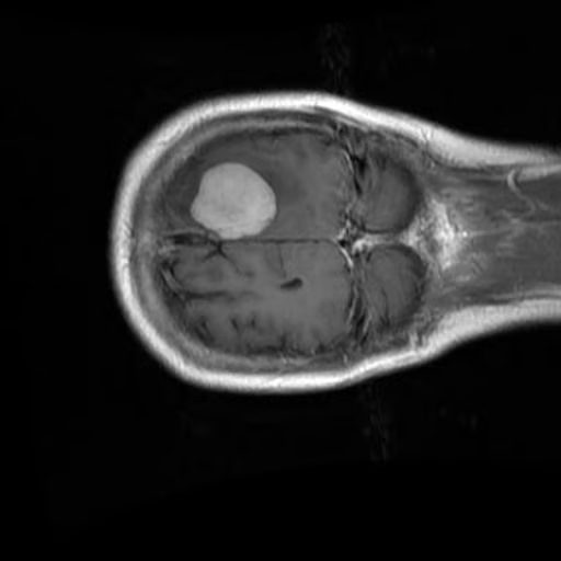

print(data["train"][0]["label"])

1

5. Processing the dataset

Before processing the dataset, it is important to first check the names of the labels to ensure proper handling of the classification task.

BRAIN_CANCER_CLASSES = data["train"].features["label"].names
print("Detected classes:", BRAIN_CANCER_CLASSES)

The detected classes are: ['brain_glioma', 'brain_menin', 'brain_tumor'].

Detected classes: ['brain_glioma', 'brain_menin', 'brain_tumor']

To enhance the classification process, we will modify these class labels by adding a prefix (A, B, C) for better organization and to align with a custom prompt format. 

BRAIN_CANCER_CLASSES = ['A: brain glioma', 'B: brain menin', 'C: brain tumor']

Next, we create a custom prompt that will be used to guide the model during fine-tuning. The prompt includes the updated class labels.

options = "\n".join(BRAIN_CANCER_CLASSES)
PROMPT = f"What is the most likely type of brain cancer shown in the MRI image?\n{options}"

To prepare the dataset for fine-tuning, we will create a new column called "messages". This column will contain structured data representing a user query (the prompt) and assistant response (the correct label). 

def format_data(example: dict[str, any]) -> dict[str, any]:
    example["messages"] = [
        {
            "role": "user",
            "content": [
                {
                    "type": "image",
                },
                {
                    "type": "text",
                    "text": PROMPT,
                },
            ],
        },
        {
            "role": "assistant",
            "content": [
                {
                    "type": "text",
                    "text": BRAIN_CANCER_CLASSES[example["label"]],
                },
            ],
        },
    ]
    return example

# Apply the formatting to the dataset
formatted_data = data.map(format_data)

To verify the formatting, we can inspect the message column from the first sample:

formatted_data["train"][0]["messages"]

The resulting formatted data point looks like this:

[{'content': [{'text': None, 'type': 'image'},
   {'text': 'What is the most likely type of brain cancer shown in the MRI image?\nA: brain glioma\nB: brain menin\nC: brain tumor',
    'type': 'text'}],
  'role': 'user'},
 {'content': [{'text': 'B: brain menin', 'type': 'text'}],
  'role': 'assistant'}]

Fine-Tuning MedGemma on the Brain MRI Dataset

In this section, we will fine-tune the MedGemma 4B Instruct model on the Brain MRI dataset. This involves downloading the model and processor, setting up the LoRA adapter, configuring the trainer, and starting the training process.

6. Loading the model and tokenizer

Since MedGemma is a gated model, you need to log in to the Hugging Face CLI using your API key. This also allows you to save your fine-tuned model to the Hugging Face Hub. Check out our course, Working with Hugging Face: Your Guide to the Hub, if you need a refresher. 

from huggingface_hub import login
import os

hf_token = os.environ.get("HF_TOKEN")
login(hf_token)

We use the Transformers library to load the MedGemma 4B Instruct model and its processor. The model is configured to use bfloat16 precision for efficient computation on GPUs.

import torch
from transformers import AutoProcessor, AutoModelForImageTextToText, BitsAndBytesConfig

model_id = "google/medgemma-4b-it"

# Check if GPU supports bfloat16
if torch.cuda.get_device_capability()[0] < 8:
    raise ValueError("GPU does not support bfloat16, please use a GPU that supports bfloat16.")

model_kwargs = dict(
    attn_implementation="eager",
    torch_dtype=torch.bfloat16,
    device_map="auto",
)

model = AutoModelForImageTextToText.from_pretrained(model_id, **model_kwargs)
processor = AutoProcessor.from_pretrained(model_id)

# Use right padding to avoid issues during training
processor.tokenizer.padding_side = "right"

7. Setting up the model

To fine-tune the MedGemma 4B Instruct model efficiently, we will use Low-Rank Adaptation (LoRA), a parameter-efficient fine-tuning method. 

LoRA allows us to adapt large models by training only a small number of additional parameters, significantly reducing computational costs while maintaining performance. 

from peft import LoraConfig

peft_config = LoraConfig(
    lora_alpha=16,
    lora_dropout=0.05,
    r=16,
    bias="none",
    target_modules="all-linear",
    task_type="CAUSAL_LM",
    modules_to_save=[
        "lm_head",
        "embed_tokens",
    ],
)

To handle both image and text inputs during training, we define a custom collation function. This function processes the dataset examples into a format suitable for the model, including tokenizing text and preparing image data.

def collate_fn(examples: list[dict[str, any]]):
    texts = []
    images = []
    for example in examples:
        images.append([example["image"]])
        texts.append(
            processor.apply_chat_template(
                example["messages"], add_generation_prompt=False, tokenize=False
            ).strip()
        )

    # Tokenize the texts and process the images
    batch = processor(text=texts, images=images, return_tensors="pt", padding=True)

    # The labels are the input_ids, with the padding and image tokens masked in
    # the loss computation
    labels = batch["input_ids"].clone()

    # Mask image tokens
    image_token_id = [
        processor.tokenizer.convert_tokens_to_ids(
            processor.tokenizer.special_tokens_map["boi_token"]
        )
    ]
    # Mask tokens that are not used in the loss computation
    labels[labels == processor.tokenizer.pad_token_id] = -100
    labels[labels == image_token_id] = -100
    labels[labels == 262144] = -100

    batch["labels"] = labels
    return batch

We use the SFTConfig class from the trl library to define the training arguments. These arguments control the fine-tuning process, including batch size, learning rate, and gradient accumulation steps.

from trl import SFTConfig

args = SFTConfig(
    output_dir="medgemma-brain-cancer",            
    num_train_epochs=1,                       
    per_device_train_batch_size=8,                           
    per_device_eval_batch_size=8,                            
    gradient_accumulation_steps=8,                           
    gradient_checkpointing=True,                             
    optim="adamw_torch_fused",                               
    logging_steps=0.1,                                        
    save_strategy="epoch",                                   
    eval_strategy="steps",                                   
    eval_steps=0.1,                                           
    learning_rate=2e-4,                             
    bf16=True,                                               
    max_grad_norm=0.3,                                       
    warmup_ratio=0.03,                                       
    lr_scheduler_type="linear",                              
    push_to_hub=True,                                        
    report_to="none",
    gradient_checkpointing_kwargs={"use_reentrant": False},  
    dataset_kwargs={"skip_prepare_dataset": True},           
    remove_unused_columns = False,                           
    label_names=["labels"],                                  
)

The SFTTrainer simplifies the fine-tuning process by combining the model, dataset, data collator, training arguments, and LoRA configuration into a single workflow. This makes the process streamlined and user-friendly.

from trl import SFTTrainer

trainer = SFTTrainer(
    model=model,
    args=args,
    train_dataset=formatted_data["train"],
    eval_dataset=formatted_data["validation"].shuffle().select(range(50)), 
    peft_config=peft_config,
    processing_class=processor,
    data_collator=collate_fn,
)

8. Model training

Once the model, dataset, and training configurations are set up, we can begin the fine-tuning process. The SFTTrainer simplifies this step, allowing us to train the model with just a single command:

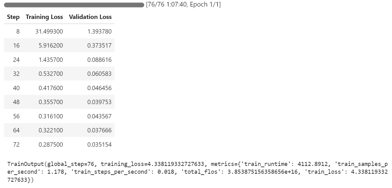
trainer.train()

The training process took approximately 1 hour and 8 minutes to complete. During this time, the training loss and validation loss steadily decreased with each step, indicating that the model was learning effectively.

After the training is complete, the fine-tuned model can be saved locally and pushed to the Hugging Face Hub using the save_model() method. 

trainer.save_model()

The model is now available kingabzpro/medgemma-brain-cancer · Hugging Face

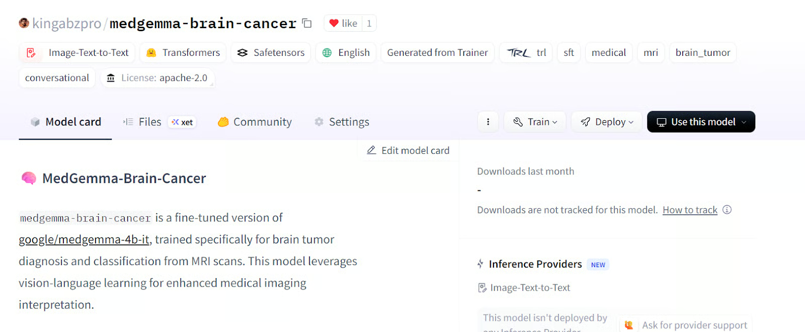
Source kingabzpro/medgemma-brain-cancer

Model Evaluation

To evaluate the performance of the MedGemma 4B model, we will test both the base model and the fine-tuned model on the validation dataset. This process involves clearing the memory, preparing the test data, generating the response, and calculating key metrics such as accuracy and F1 score. 

Before starting the evaluation, we remove the training setup to free up GPU memory and ensure a clean environment for testing

del model
del trainer
torch.cuda.empty_cache()

9. Setting up for model testing

We format the validation dataset to match the input structure required by the model. This involves creating a "messages" column that contains the user prompt for each example.

def format_test_data(example: dict[str, any]) -> dict[str, any]:
    example["messages"] = [
        {
            "role": "user",
            "content": [
                {
                    "type": "image",
                },
                {
                    "type": "text",
                    "text": PROMPT,
                },
            ],
        },
    ]
    return example

test_data = data["validation"]
test_data = test_data.map(format_test_data)

To evaluate the performance of the model, we use the evaluate library, which provides pre-built metrics for tasks like classification. After importing the library and loading the necessary metrics, we extract ground-truth labels from the test dataset. A helper function, compute_metrics, is then defined to calculate accuracy and F1 score by comparing the predictions to these labels.

import evaluate

accuracy_metric = evaluate.load("accuracy")
f1_metric = evaluate.load("f1")

# Ground-truth labels
REFERENCES = test_data["label"]


def compute_metrics(predictions: list[int]) -> dict[str, float]:
    metrics = {}
    metrics.update(
        accuracy_metric.compute(
            predictions=predictions,
            references=REFERENCES,
        )
    )
    metrics.update(
        f1_metric.compute(
            predictions=predictions,
            references=REFERENCES,
            average="weighted",
        )
    )
    return metrics

To ensure consistency in label handling, we cast the "label" column of the dataset to a ClassLabel type. This allows for efficient mapping between label indices and their corresponding names. Additionally, we define alternative label mappings to handle variations in label formatting during post processing.

from datasets import ClassLabel

test_data = test_data.cast_column(
    "label",
    ClassLabel(names=BRAIN_CANCER_CLASSES)
)

LABEL_FEATURE = test_data.features["label"]

ALT_LABELS = dict([
    (label, f"({label.replace(': ', ') ')}") for label in BRAIN_CANCER_CLASSES
])

To map the model's predictions to the correct class labels, we define a postprocess function. This function ensures that predictions are matched to the appropriate label, accounting for both canonical and alternative label formats.

def postprocess(prediction, do_full_match: bool = False) -> int:
    if isinstance(prediction, str):
        response_text = prediction
    else:
        response_text = prediction[0]["generated_text"]

    if do_full_match:
        return LABEL_FEATURE.str2int(response_text)

    for label in BRAIN_CANCER_CLASSES:
        # accept canonical or alternative wording
        if label in response_text or ALT_LABELS[label] in response_text:
            return LABEL_FEATURE.str2int(label)

    return -1

10. Model performance on the base model

To evaluate the base model's performance, we load the pre-trained model and processor, configure the generation settings, and prepare the prompts and images for testing.

import torch
from transformers import AutoModelForImageTextToText, AutoProcessor

model_kwargs = dict(
    torch_dtype=torch.bfloat16,
    device_map="auto",
)

model = AutoModelForImageTextToText.from_pretrained(
    model_id, **model_kwargs
)

from transformers import GenerationConfig
gen_cfg = GenerationConfig.from_pretrained(model_id)
gen_cfg.update(
    do_sample          = False, 
    top_k              = None, 
    top_p              = None,
    cache_implementation = "dynamic" 
)
model.generation_config = gen_cfg

processor  = AutoProcessor.from_pretrained(args.output_dir)
tok = processor.tokenizer

model.config.pad_token_id            = tok.pad_token_id
model.generation_config.pad_token_id = tok.pad_token_id

def chat_to_prompt(chat_turns):
    return processor.apply_chat_template(
        chat_turns,
        add_generation_prompt=True,   # tells the model "your turn"
        tokenize=False                # we want raw text, not ids
    )

prompts = [chat_to_prompt(c) for c in test_data["messages"]]
images  = test_data["image"]                         # already a list of PIL images
assert len(prompts) == len(images), "1 prompt must match 1 image!"

We have created a batch_predict function that processes the test dataset in batches. This function generates predictions for each prompt-image pair and applies post processing to map the outputs to the correct labels.

import torch
from typing import List, Any, Callable


def batch_predict(
    prompts,
    images,
    model,
    processor,
    postprocess,
    *,
    batch_size=64,
    device="cuda",
    dtype=torch.bfloat16,
    **gen_kwargs
):
    preds = []
    for i in range(0, len(prompts), batch_size):
        texts = prompts[i : i + batch_size]
        imgs = [[img] for img in images[i : i + batch_size]]
        enc = processor(text=texts, images=imgs, padding=True, return_tensors="pt").to(
            device, dtype=dtype
        )
        lens = enc["attention_mask"].sum(dim=1)
        with torch.inference_mode():
            out = model.generate(
                **enc,
                disable_compile=True,
                **gen_kwargs
            )
        for seq, ln in zip(out, lens):
            ans = processor.decode(seq[ln:], skip_special_tokens=True)
            preds.append(postprocess(ans))
    return preds

We will use the batch_predict function to generate predictions for the base model on the test dataset. The predictions are then evaluated using the compute_metrics function.

bf_preds = batch_predict(
    model         = model,
    processor     = processor,
    prompts       = prompts,
    images        = images,
    batch_size    = 64,
    max_new_tokens= 40,          # forwarded to generate
    postprocess= postprocess, # your label-mapping function
)




bf_metrics = compute_metrics(bf_preds)
print(f"Baseline metrics: {bf_metrics}")

The result is not impressive. We got 33% accuracy, which is quite bad. 

Baseline metrics: {'accuracy': 0.33745874587458746, 'f1': 0.1737287617650654}

To better understand the model's behavior, we can generate predictions for a single example from the dataset. This involves creating a helper function to process the input and return the model's response.

The predict_one function takes a prompt and an image as input, processes them using the model's processor, and generates a response. The function ensures that the model's output is decoded into human-readable text.

import torch
from typing import Union, Dict, Any, List
from transformers import AutoModelForImageTextToText, AutoProcessor


def predict_one(
    prompt,
    image,
    model,
    processor,
    *,
    device="cuda",
    dtype=torch.bfloat16,
    disable_compile=True,
    **gen_kwargs
) -> str:
    inputs = processor(text=prompt, images=image, return_tensors="pt").to(
        device, dtype=dtype
    )
    plen = inputs["input_ids"].shape[-1]
    with torch.inference_mode():
        ids = model.generate(
            **inputs,
            disable_compile=disable_compile,
            **gen_kwargs
        )
    return processor.decode(ids[0, plen:], skip_special_tokens=True)

We will use the predict_one to generate a response for the 11th sample from the dataset. This involves preparing the prompt and running the prediction function.

idx     = 10
chat    = test_data["messages"][idx]
prompt  = processor.apply_chat_template(
            chat,
            add_generation_prompt=True,
            tokenize=False
          )

# run the one-sample helper
answer = predict_one(
    prompt   = prompt,
    image    = test_data["image"][idx],
    model    = model,
    processor= processor,
    max_new_tokens = 40 
)

print("Model answer:", answer)

As a result, we received a lengthy sentence explaining why the brain glioma was chosen. The response is completely wrong, even the classification is wrong.

Model answer: Based on the MRI image, the most likely type of brain cancer is **A: brain glioma**.

Here's why:

*   **Gliomas** are a common type of brain tumor

11. Model performance on the fine-tuned model

To evaluate the fine-tuned model, we repeat the evaluation process by loading the model from the output directory, generating predictions, and calculating metrics.

We load the fine-tuned model and processor from the output directory, run the batch_predict function, and calculate the metrics. 

model = AutoModelForImageTextToText.from_pretrained(
    args.output_dir, **model_kwargs
)
model.generation_config = gen_cfg

processor  = AutoProcessor.from_pretrained(args.output_dir)
tok = processor.tokenizer

model.config.pad_token_id            = tok.pad_token_id
model.generation_config.pad_token_id = tok.pad_token_id

af_preds = batch_predict(
    model         = model,
    processor     = processor,
    prompts       = prompts,
    images        = images,
    batch_size    = 64,
    max_new_tokens= 40,          # forwarded to generate
    postprocess= postprocess, # your label-mapping function
)
af_metrics = compute_metrics(af_preds)
print(f"Fine-tuned metrics: {af_metrics}")

These results show a significant improvement over the base model, highlighting the effectiveness of fine-tuning. The accuracy jumped from 33% to 89% with only 1 epoch. 

Fine-tuned metrics: {'accuracy': 0.8927392739273927, 'f1': 0.892641793935792}

To further analyze the fine-tuned model's performance, we generate a prediction for a single example from the test dataset.

idx     = 10
chat    = test_data["messages"][idx]
prompt  = processor.apply_chat_template(
            chat,
            add_generation_prompt=True,
            tokenize=False
          )

# run the one-sample helper
answer = predict_one(
    prompt   = prompt,
    image    = test_data["image"][idx],
    model    = model,
    processor= processor,
    max_new_tokens = 40              # any generate-kwargs you need
)

print("Model answer:", answer)

The model produced the result in a clear and precise manner, with the classification being both accurate and well-structured.

Model answer: C: brain tumor

If you are facing issues running the above code, please refer to the companion notebook: Fine_tuning_MedGemma.ipynb

Conclusion

MedGemma represents a significant step forward in using AI for medical sciences. By empowering doctors and physicians to make faster and more accurate judgments, it enables quicker diagnoses and more effective treatment plans for patients. 

Fine-tuning vision language models like MedGemma 4B Instruct allows for adaptability across various medical tasks, from image classification to integrating reasoning capabilities. 

In this tutorial, we have learned how to fine-tune a vision-language model on a Brain MRI dataset for brain cancer classification. The results were remarkable, with the model's accuracy improving from 33% to 89%, a substantial leap that highlights the potential of fine-tuning in medical AI applications.

If you’re interested in learning more, I recommend checking out these resources: 

• Biomedical Image Analysis in Python course
• Deep Learning for Images with PyTorch course
• Fine-Tuning Your Own Llama 3 Model code-along