Fisher’s Exact Test: Making Decisions with Small Samples

Organizations make decisions every day based on how customers behave, how products perform, and how operations fluctuate. To ensure these decisions are based on genuine underlying relationships and patterns in data, analysts frequently use statistical tests. 

While common statistical tests work well for large datasets, businesses don’t always have the luxury of working with large datasets. In fact, many decisions have to be made using small sample sizes, niche customer segments, or rare events. In these situations, traditional tests, like chi-square, may fall short, either producing misleading results or lacking the precision required to confidently act on the insights. 

This is where Fisher’s exact test becomes valuable. Keep reading and I'll show you how.

What Is Fisher's Exact Test?

Fisher's exact test is used to evaluate the association between categorical variables when data is limited. It is most often applied to 2×2 contingency tables, and it calculates the exact probability of observing data as extreme as what was collected, assuming the null hypothesis of independence is true.

An analyst might use Fisher's exact test, for example, when evaluating the effectiveness of a targeted marketing campaign. If, for example, the analyst were testing the effectiveness of an email vs. social media campaign, and this was for a niche customer group with small sample sizes, he or she might create a contingency table and run Fisher's exact test. Or else, in a quality control setting, an analyst could use the test to address challenges in incident reporting and defect tracking. When certain failure types occur only a few times, Fisher's exact test can assess whether factors such as machine type are genuinely linked to defect occurrences.

Statistical Theory and Mathematical Foundation

Having developed an intuitive sense of why the test is important, we can now formalize it. At its core, Fisher’s exact test is a statistical method used to determine whether there is a non-random association between two categorical variables. It is most commonly applied to 2×2 contingency tables to compare two groups across two outcomes, for example, “treatment versus control” against “improved versus not improved.”

Interestingly, its origins trace back to one of the most famous stories in statistics, known as the “lady tasting tea” experiment. Sir Ronald A. Fisher designed an experiment to evaluate Dr. Muriel Bristol’s claim that she could distinguish whether milk or tea had been poured into a cup first purely by taste. As part of the experiment, Fisher arranged eight cups and asked her to identify which were “milk-first” versus “tea-first”. Due to the small sample size, Fisher developed an exact method for determining whether the pattern of correct guesses could have occurred by chance, laying the foundation for what we now know as Fisher’s exact test.

In situations where data are limited, imbalanced, or difficult to obtain, much like in clinical research, Fisher's test helps determine whether treatments and outcomes are associated in a meaningful way. Ecology, epidemiology, genetics, and quality control are some of the fields that involve sparse data and rely on this test.

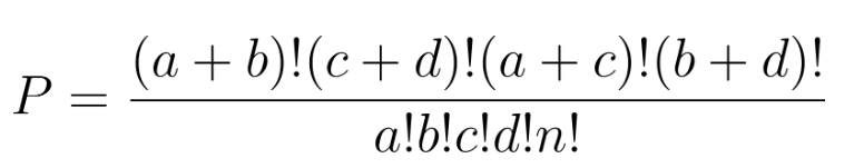
Fisher’s exact test evaluates independence by computing exact hypergeometric probabilities. For a 2×2 table:

The probability of observing that exact configuration under the null hypothesis (no association) is calculated with the hypergeometric distribution:

Tests can be one-sided, such as answering “Is A1 more likely in B1 than B2?” or two-sided: “Any association at all?” Unlike large-sample approximations (e.g., chi-squared), Fisher’s method ensures accuracy even when expected frequencies are low.

Assumptions and Prerequisites

To apply Fisher’s exact test, we need to have the following conditions.

• Data must be categorical
• Presented in a 2×2 contingency table
• Observations are independent
• Margins (row & column totals) are fixed under the null

Fisher’s test is preferred when any of the expected counts in the grid are extremely low (less than 5), or the results are sparse or heavily unbalanced.

Fisher's Exact Test in Python

Suppose we test whether a drug improves recovery:

Here are the hypotheses:

• H₀: Treatment and recovery are independent
• H₁: Treatment improves recovery (one-sided)

And here is how I would consider this in Python:

from scipy.stats import fisher_exact

# Construct contingency table
table = [[8, 2],
         [4, 11]]

oddsratio, p_value = fisher_exact(table, alternative='two-sided')
print("Odds Ratio:", oddsratio)
print("Two-sided p-value:", round(p_value, 2))

# One-sided test (treatment better)
_, p_value_one = fisher_exact(table, alternative='greater')
print("One-sided p-value:", round(p_value_one, 2))

Odds Ratio: 11.0
Two-sided p-value: 0.02
One-sided p-value: 0.01

A small p-value of 0.02 suggests a real association between treatment and recovery.

Now, let’s pick a real-life example using NHANES 2017–2018 public data to examine the association between “current smoking status” and “ever being told you have asthma” in adults.

Files used (all from the NHANES official site):

• DEMO_J.XPT — Demographics (age, sex, weights, etc.)

• SMQ_J.XPT — Smoking - Cigarette Use (smoking history & current use)

• MCQ_J.XPT — Medical Conditions (including "ever told you had asthma")

Below are the steps we are going to follow:

1. Download and load the datasets

2. Create binary variables:

1. current_smoker (yes/no)

2. asthma_ever (yes/no)

3. Build a 2×2 contingency table

4. Run Fisher’s exact test (two-sided and one-sided)

5. Compute a 95% confidence interval for the odds ratio

6. Interpret the results

Note: Proper NHANES analysis requires survey weights and a complex design.

Here, we ignore weights for didactic purposes. Let’s import the required libraries.

# %% Imports
import pandas as pd
import numpy as np
from scipy.stats import fisher_exact
from statsmodels.stats.contingency_tables import Table2x2

Let us manually download the XPT files from CDC and put them in a local data/ folder:

• Go to:

• Demographics: 2017–2018 Demographics Data (DEMO_J)

• Medical Conditions: MCQ_J

• Smoking - Cigarette Use: SMQ_J

• Download:

• DEMO_J Data [XPT]

• MCQ_J Data [XPT]

• SMQ_J Data [XPT]

• Save them as:

• data/DEMO_J.XPT

• data/MCQ_J.XPT

• data/SMQ_J.XPT

# Set paths or URLs here.
# If you've downloaded locally, point to the local paths:
DEMO_PATH = "data/DEMO_J.XPT"
MCQ_PATH  = "data/MCQ_J.XPT"
SMQ_PATH  = "data/SMQ_J.XPT"

# If you prefer to read directly from URLs, uncomment these instead:
# DEMO_PATH = "https://wwwn.cdc.gov/Nchs/NHanes/2017-2018/DEMO_J.XPT"
# MCQ_PATH  = "https://wwwn.cdc.gov/Nchs/NHanes/2017-2018/MCQ_J.XPT"
# SMQ_PATH  = "https://wwwn.cdc.gov/Nchs/NHanes/2017-2018/SMQ_J.XPT"

# Read SAS transport (.XPT) files
demo = pd.read_sas(DEMO_PATH, format="xport")
mcq  = pd.read_sas(MCQ_PATH,  format="xport")
smq  = pd.read_sas(SMQ_PATH,  format="xport")

demo.head()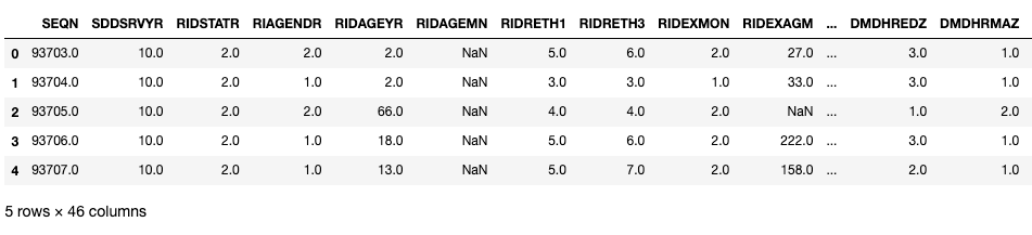

mcq.head()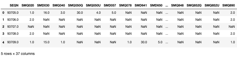

smq.head()

Let’s look at some key variables in these DataFrames. Here, SEQN is the respondent ID and can be used as a join key.

# %% Inspect key variables

# SEQN is the respondent ID present in all three files.
# Check columns and pick what we need:
print("DEMO columns (subset):", demo.columns[:10])
print("MCQ columns (subset):", mcq.columns[:10])
print("SMQ columns (subset):", smq.columns[:10])

DEMO columns (subset): Index(['SEQN', 'SDDSRVYR', 'RIDSTATR', 'RIAGENDR', 'RIDAGEYR', 'RIDAGEMN',
       'RIDRETH1', 'RIDRETH3', 'RIDEXMON', 'RIDEXAGM'],
      dtype='object')
MCQ columns (subset): Index(['SEQN', 'MCQ010', 'MCQ025', 'MCQ035', 'MCQ040', 'MCQ050', 'AGQ030',
       'MCQ053', 'MCQ080', 'MCQ092'],
      dtype='object')
SMQ columns (subset): Index(['SEQN', 'SMQ020', 'SMD030', 'SMQ040', 'SMQ050Q', 'SMQ050U', 'SMD057',
       'SMQ078', 'SMD641', 'SMD650'],
      dtype='object')

Let’s filter for the required columns and also filter by age (greater than 20). 

# %% Keep only necessary variables and filter adults

demo_sub = demo[["SEQN", "RIDAGEYR", "RIAGENDR"]].copy()
mcq_sub  = mcq[["SEQN", "MCQ010"]].copy()
smq_sub  = smq[["SEQN", "SMQ040"]].copy()

# Merge on SEQN (inner join: keep only participants present in all three files)
df = (
    demo_sub
    .merge(mcq_sub, on="SEQN", how="inner")
    .merge(smq_sub, on="SEQN", how="inner")
)
# Restrict to adults aged 20+
df = df[df["RIDAGEYR"] >= 20].copy()
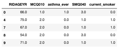
df.head()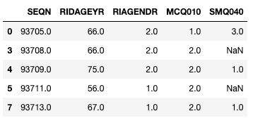

MCQ010 represents patients with Asthma conditions, where the value of 1 is Yes and 2 means No. Similarly, SMQ040 shows whether the respondent is a smoker or not. 

# %% Recode variables into binary indicators

# 1. Asthma: MCQ010
#    1 = Yes, 2 = No, 7 = Refused, 9 = Don't know
#    We'll create asthma_ever: 1 = yes, 0 = no, NaN otherwise

df["asthma_ever"] = np.nan
df.loc[df["MCQ010"] == 1, "asthma_ever"] = 1
df.loc[df["MCQ010"] == 2, "asthma_ever"] = 0

# 2. Current smoker: SMQ040
#    1 = Every day, 2 = Some days, 3 = Not at all, 7/9 = missing
#    We'll create current_smoker: 1 = yes (1 or 2), 0 = no (3), NaN otherwise

df["current_smoker"] = np.nan
df.loc[df["SMQ040"].isin([1, 2]), "current_smoker"] = 1
df.loc[df["SMQ040"] == 3, "current_smoker"] = 0

# Drop rows with missing recodes
df_clean = df.dropna(subset=["asthma_ever", "current_smoker"]).copy()
df_clean[["RIDAGEYR", "MCQ010", "asthma_ever", "SMQ040", "current_smoker"]].head()

We create new columns, asthma_ever and current_smoker

Let’s create the contingency table so that we can use Fisher’s Exact Test.

# %% Build a 2×2 contingency table

# Ensure ints
df_clean["asthma_ever"] = df_clean["asthma_ever"].astype(int)
df_clean["current_smoker"] = df_clean["current_smoker"].astype(int)

contingency = pd.crosstab(
    df_clean["current_smoker"],
    df_clean["asthma_ever"],
    rownames=["Current smoker (1=yes,0=no)"],
    colnames=["Ever told asthma (1=yes,0=no)"]
)
contingency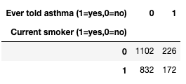

Convert the contingency table to a NumPy array.

# %% Fisher's Exact Test

# Convert to 2x2 numpy array with explicit ordering:
# rows: [non-smoker, smoker] ; cols: [no asthma, asthma]
table = np.array([
    [contingency.loc[0, 0], contingency.loc[0, 1]],
    [contingency.loc[1, 0], contingency.loc[1, 1]]
])

table

array([[1102,  226],
       [ 832,  172]])

Finally, run two-sided and one-sided Fisher’s Exact Tests.

# Run Fisher's exact test (two-sided and one-sided)
oddsratio, p_two_sided = fisher_exact(table, alternative="two-sided")
_, p_smoker_higher_asthma = fisher_exact(table, alternative="greater")
_, p_smoker_lower_asthma  = fisher_exact(table, alternative="less")

print("2x2 table (rows: non-smoker, smoker; cols: no asthma, asthma)")
print(table)
print()
print(f"Odds ratio (Fisher): {oddsratio:.3f}")
print(f"Two-sided p-value: {p_two_sided:.5f}")
print(f"One-sided p-value (H1: smokers have higher asthma odds): {p_smoker_higher_asthma:.5f}")
print(f"One-sided p-value (H1: smokers have lower asthma odds): {p_smoker_lower_asthma:.5f}")

2x2 table (rows: non-smoker, smoker; cols: no asthma, asthma)
[[1102  226]
 [ 832  172]]

Odds ratio (Fisher): 1.008
Two-sided p-value: 0.95571
One-sided p-value (H1: smokers have higher asthma odds): 0.49274
One-sided p-value (H1: smokers have lower asthma odds): 0.55144

High p-values show that there is no evidence of a statistically significant association between current smoking and ever having been diagnosed with asthma in this sample.

The odds ratio ~1 means that current smokers have virtually the same odds of reporting an asthma diagnosis as non-smokers. Any difference observed is well within what could occur by random chance.

Comparison with Alternative Statistical Methods

Different statistical tests are used for analyzing relationships in contingency tables depending on sample size, data structure, and assumptions:

Fisher’s exact test

Best for small samples and when some expected cell counts are low. It provides exact p-values, making it very reliable, but it can become computationally slow as tables get large.

Chi-squared test

The standard choice for large sample sizes. It’s fast, common, and easy to apply, but it becomes inaccurate when expected counts fall below 5 due to its reliance on approximations.

Barnard’s exact test

A more powerful alternative to Fisher’s test in 2×2 tables. It does not assume fixed margins, which can make results more sensitive, but the method is less widely implemented in software.

McNemar’s test

Designed for paired or matched categorical data (e.g., pre- vs. post-treatment in the same subjects). It accounts for dependence between observations, but cannot be used when data points are independent.

Computational Considerations

Performance can be a concern with Fisher’s exact test because computations scale poorly when moving beyond simple 2×2 contingency tables. While the Freeman–Halton extension allows the test to be applied to 2×3 and 3×3 tables, the computational cost increases rapidly as the size of the table grows. As a result, efficient algorithms and optimizations are especially important in fields like genetics and clinical research, where exact testing may need to be performed repeatedly on many small but complex datasets.

Interpretation & Statistical Reporting

When interpreting and reporting Fisher’s exact test results, it is important to include the exact p-value, provide the odds ratio along with a 95% confidence interval, and clearly state whether a one- or two-sided test was performed. Results should also be supported with a practical context to help readers understand the real-world significance of the findings. For example, one might write: “Fisher’s exact test showed a significant association between treatment and recovery (OR=11.0, p=0.02, two-tailed).”

Extensions and Advanced Applications

Extensions and advanced applications of Fisher’s exact test help address more complex data scenarios and improve accuracy when dealing with small or sparse datasets. The Freeman–Halton extension allows the test to be applied to larger contingency tables beyond the standard 2×2 format, such as 2×3 or 3×3 tables. The mid-P exact test offers a less conservative alternative to Fisher’s test, improving statistical power while still maintaining reliability. Bayesian exact tests incorporate prior knowledge into the analysis, making them particularly useful when data are limited or when expert judgment can guide inference. Additionally, bias correction methods for odds ratios provide more accurate effect size estimates in studies with small sample sizes or zero counts, ensuring better interpretation of the strength and direction of associations.

Limitations and Methodological Considerations

Fisher’s exact test can be conservative, which may reduce statistical power and make it harder to detect real effects, especially in small studies. When data are very sparse, interpreting results can be challenging because confidence intervals widen and estimates become unstable. Additionally, applying the test repeatedly across many variables increases the risk of false discoveries, so careful control for multiple testing is important.

Visualizing Contingency Tables

Good visualization options for presenting contingency table results include stacked bar charts, side-by-side bar charts, and mosaic plots. These visuals help clearly communicate the relationship between categorical variables and make patterns or group differences easier to interpret.

Here is a Python example:

import seaborn as sns
import matplotlib.pyplot as plt
import pandas as pd

df = pd.DataFrame({
    "Outcome": ["Recovered", "Not Recovered"] * 2,
    "Count": [8, 2, 4, 11],
    "Group": ["Treatment"] * 2 + ["Control"] * 2
})

sns.barplot(data=df, x="Outcome", y="Count", hue="Group")
plt.title("Treatment Outcomes")
plt.show()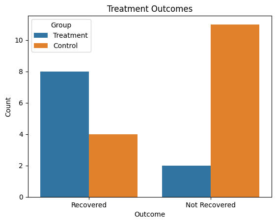

Conclusion

Fisher’s exact test remains a gold standard for analyzing small categorical datasets. Born from a teacup in a garden, it has since evolved into an important and widely used tool in medicine, genetics, human subjects research, and business experimentation.

Enroll in our Statistics Fundamentals in Python skill track to keep learning which, in addition to hypothesis testing, will help you practice statistical model building with linear and logistic regression.