When working with real-world data, it's often the case that sample sizes are small or population variance is unknown. These are the conditions where traditional statistical techniques based on the normal distribution may not hold. That’s where the t-distribution, also known as Student’s t-distribution, becomes useful. It’s a powerful tool for making reliable statistical inferences when data is limited or uncertainty is high.
In this article, we’ll study what the t-distribution is, how it compares to similar distributions, its key mathematical properties, and how it is used in practice, particularly in hypothesis testing and confidence intervals. I’ve also included a t-distribution table at the end for quick reference.
What Is the T-Distribution?
Much like the normal distribution, the t-distribution is also symmetrical and bell-shaped. However, it has heavier tails that reflect greater uncertainty that often comes with smaller sample sizes.
Besides, there's another key factor that sets the t-distribution apart: it is defined by its degrees of freedom (df). This value, df, is calculated as the sample size minus one (n − 1) and influences the shape of the distribution.
As the degrees of freedom increase, the t-distribution becomes more similar to the normal distribution. When the sample size is large (e.g., n > 30), the difference becomes so small that the t-distribution starts resembling the standard normal curve.
T-Distribution vs. Other, Similar Distributions
It's helpful to compare the t-distribution to other, similar ones.
T-distribution vs. normal distribution
While we've noted that both distributions are bell-shaped, with the t-distribution having heavier tails and being more suitable for small samples and unknown population variance, it's especially important to highlight its tolerance towards outliers.
|
Feature |
t-distribution |
Normal distribution |
|
Shape |
Bell-shaped, heavier tails |
Bell-shaped, thinner tails |
|
Use Case |
Small samples, σ unknown |
Large samples, σ known |
|
Degrees of Freedom |
Required |
Not applicable |
|
Sensitivity to Outliers |
More tolerant |
Less tolerant |
For larger samples, the central limit theorem justifies using the normal distribution, as sample means tend to follow a normal distribution regardless of the population shape.
T-distribution vs. Z-distribution
The Z-distribution refers to the standard normal distribution, which has a mean of 0 and a standard deviation of 1.
|
Feature |
t-distribution |
Z-distribution |
|
Variance Known? |
No |
Yes |
|
Tail Thickness |
Heavier |
Thinner |
|
Common Test |
T-tests |
Z-tests |
|
Use for Small Samples |
Yes |
No |
Let’s understand this with a Python code example:
import numpy as np
import matplotlib.pyplot as plt
from scipy.stats import t, norm

# X-axis range
x = np.linspace(-5, 5, 1000)

# Standard Normal (Z) Distribution
z_dist = norm.pdf(x)

# Plotting
plt.figure(figsize=(10, 6))
plt.plot(x, z_dist, label='Z-Distribution (Standard Normal)', color='black', linewidth=2)

# T-Distributions with different degrees of freedom
dfs = [1, 3, 5, 10, 30]
colors = ['red', 'orange', 'green', 'blue', 'purple']

for df, color in zip(dfs, colors):
    t_dist = t.pdf(x, df)
    plt.plot(x, t_dist, label=f'T-Distribution (df={df})', color=color, linestyle='--')

plt.title('T-Distribution vs Z-Distribution: Heavier Tails for Smaller Sample Sizes')
plt.xlabel('x')
plt.ylabel('Density')
plt.legend()
plt.grid(True)
plt.show()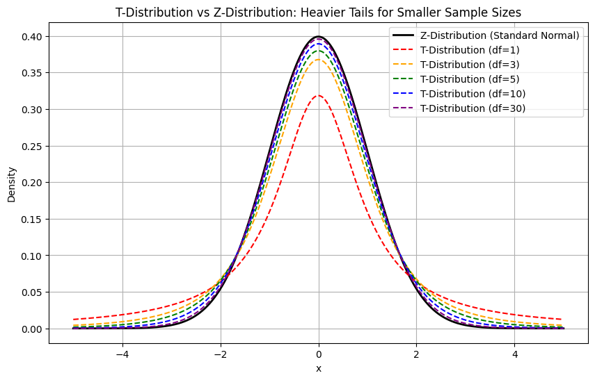
Special Cases and Related Distributions
The t-distribution is closely related to several other probability distributions:
- Standard normal distribution (as df → ∞): The t-distribution converges to the normal distribution as the degrees of freedom increase.
- Cauchy distribution (df = 1): A t-distribution with 1 degree of freedom is equivalent to the Cauchy distribution, known for having an undefined mean and variance, which effectively means that a t-distribution with one degree of freedom is rarely used in practice.
- F-distribution: The square of a t-distributed variable with ν degrees of freedom follows an F-distribution with (1, ν) degrees of freedom.
- Noncentral t-distribution: Used in power analysis and advanced statistical applications, this version incorporates a noncentrality parameter, arising when the null hypothesis is false.
Limitations of the T-Distribution
The t-distribution assumes the underlying data is approximately normally distributed. In cases of highly skewed or non-normal data, it may not be appropriate. Robust statistical techniques or nonparametric methods may be better suited in such scenarios.
Now let’s compare how the t-test behaves on normal data versus skewed data, both having the same mean.
import numpy as np
import scipy.stats as stats
import matplotlib.pyplot as plt

np.random.seed(42)

# Generate data
normal_data = np.random.normal(loc=0, scale=1, size=30)
skewed_data = np.random.exponential(scale=1.0, size=30) - 1  # Shift to mean ≈ 0

# Perform one-sample t-tests (test if mean == 0)
t_stat_normal, p_normal = stats.ttest_1samp(normal_data, popmean=0)
t_stat_skewed, p_skewed = stats.ttest_1samp(skewed_data, popmean=0)

# Plot histograms
plt.figure(figsize=(12, 5))

plt.subplot(1, 2, 1)
plt.hist(normal_data, bins=15, color='skyblue', edgecolor='black')
plt.title(f'Normal Data\np-value = {p_normal:.3f}')
plt.axvline(0, color='red', linestyle='--')

plt.subplot(1, 2, 2)
plt.hist(skewed_data, bins=15, color='salmon', edgecolor='black')
plt.title(f'Skewed Data\np-value = {p_skewed:.3f}')
plt.axvline(0, color='red', linestyle='--')

plt.suptitle("Impact of Data Shape on t-test")
plt.tight_layout()
plt.show()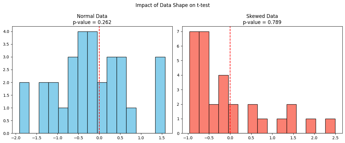
The left plot shows data from a normal distribution where the t-test is valid, and the p-value is trustworthy. Whereas the right plot shows skewed data from an exponential distribution, although the sample mean may be similar, the t-test assumes symmetry and fails to account for skew, potentially giving an inaccurate p-value.
Mathematical Properties of the T-Distribution
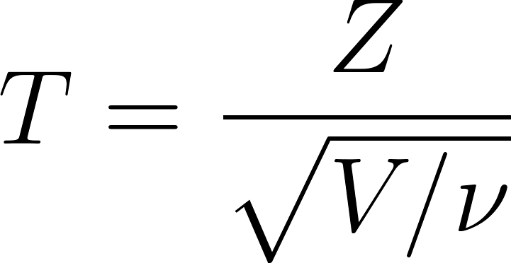
The t-distribution is defined as:
Where:
- T is the resulting value that follows a Student’s t-distribution with ν degrees of freedom
- Z is a standard normal random variable Z∼N(0,1)
- V is a chi-square distributed random variable with ν degrees of freedom, V∼χ2(ν)
- v is the degrees of freedom parameter, often equal to n−1, where is the sample size.
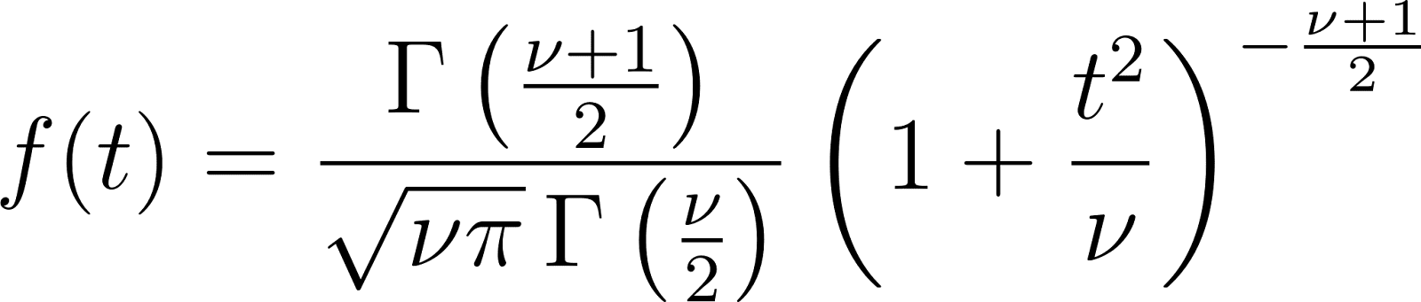
Probability density function (PDF)
Key properties
- Mean: 0 (for v > 1)
- Variance: v / (v - 2) (for v > 2)
- Skewness: 0 (symmetric distribution)
- Kurtosis: Higher than normal distribution (leptokurtic)
Simulation
Monte Carlo methods are frequently used to simulate t-distributed random variables, especially when assessing statistical significance or creating synthetic data.
Let’s simulate this using Python.
Here, our goal is to simulate a large number of small-sample experiments (sample size = 10), compute the t-statistic for each, and compare the resulting distribution to the theoretical t-distribution.
To do this, we must follow the approach below:
- Generate many samples from a normal distribution (mean = 0, std = 1).
- For each sample, compute the t-statistic: (Subtract the population mean μ from the sample mean xˉ, then divide the result by the standard error of the mean, which is the sample standard deviation divided by the square root of the sample size n)
- Plot the histogram of simulated t-values.
- Overlay the theoretical t-distribution for comparison.
import numpy as np
import matplotlib.pyplot as plt
from scipy.stats import t

# Simulation parameters
n = 10                      # sample size
mu = 0                      # population mean
sigma = 1                   # population std deviation (not used directly)
df = n - 1                  # degrees of freedom
num_simulations = 10000     # number of Monte Carlo simulations

# Monte Carlo simulation
t_stats = []
for _ in range(num_simulations):
    sample = np.random.normal(loc=mu, scale=sigma, size=n)
    sample_mean = np.mean(sample)
    sample_std = np.std(sample, ddof=1)  # sample std dev with Bessel's correction
    t_stat = (sample_mean - mu) / (sample_std / np.sqrt(n))
    t_stats.append(t_stat)

# Plot histogram of simulated t-statistics
x = np.linspace(-5, 5, 1000)
plt.figure(figsize=(10, 6))
plt.hist(t_stats, bins=50, density=True, alpha=0.6, label='Simulated t-Statistics')

# Overlay theoretical t-distribution
plt.plot(x, t.pdf(x, df), label=f'Theoretical t-Distribution (df={df})', color='red', linewidth=2)

plt.title('Monte Carlo Simulation of t-Distribution (n=10)')
plt.xlabel('t-value')
plt.ylabel('Density')
plt.legend()
plt.grid(True)
plt.show()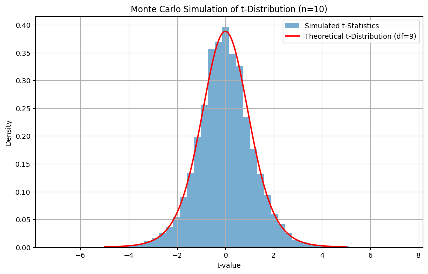
The simulated t-values form a distribution that closely matches the theoretical t-distribution with df = 9. This is a practical way to understand and validate the t-distribution through random sampling. It’s also a foundational concept behind bootstrapping and resampling-based inference.
When to Use the T-Distribution
The t-distribution is foundational in many statistical applications:
- Estimating population means when the standard deviation is unknown
- Hypothesis testing using t-tests
- Confidence intervals for small samples
- Regression analysis, where coefficients follow a t-distribution
- Bayesian inference, particularly when variance parameters are marginalized
Confidence intervals with the t-distribution
A confidence interval for the mean is calculated as:
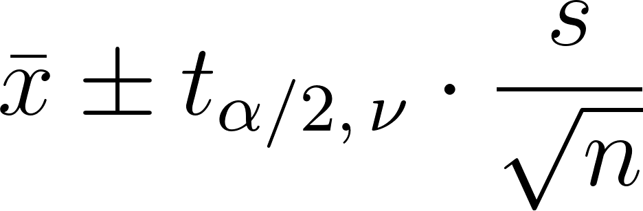
Where:
- x is the sample mean
- s is the sample standard deviation
- n is the sample size
- And the middle part is the critical value from the t-distribution. (alpha is the significance level, and alpha divided by two is because it's two-tailed.)
Use a t-distribution table or calculator to find the critical value.
Hypothesis testing with the t-distribution
In t-tests, the test statistic is:
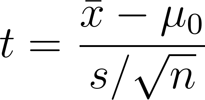
You compare this against a critical t-value to accept or reject the null hypothesis. T-tests can be:
- One-sample
- Two-sample
- Paired-sample
Graphical illustrations help visualize the critical regions in one-tailed and two-tailed tests.
T-Distribution Table
A t-distribution table lists critical values of the t-distribution for various confidence levels and degrees of freedom. It's essential for:
- Determining confidence intervals
- Conducting t-tests
- Verifying significance in regression
If it's helpful, I've included a condensed version of a t-distribution table you can refer to here:
| df | 80% (1-tailed) | 90% (2-tailed) | 95% (2-tailed) | 98% (2-tailed) | 99% (2-tailed) |
|---|---|---|---|---|---|
| 1 | 3.078 | 6.314 | 12.706 | 31.821 | 63.657 |
| 2 | 1.886 | 2.920 | 4.303 | 6.965 | 9.925 |
| 5 | 1.476 | 2.015 | 2.571 | 3.365 | 4.032 |
| 10 | 1.372 | 1.812 | 2.228 | 2.764 | 3.169 |
| 20 | 1.325 | 1.725 | 2.086 | 2.528 | 2.845 |
| 30 | 1.310 | 1.697 | 2.042 | 2.457 | 2.750 |
| 60 | 1.296 | 1.671 | 2.000 | 2.390 | 2.660 |
| ∞ | 1.282 | 1.645 | 1.960 | 2.326 | 2.576 |
Conclusion
I hope this article has provided you with a sound understanding of the t-distribution and helped bridge the gap between theory and practice. It is a core concept in statistics that deals with uncertainty, especially with small sample sizes or unknown population parameters.
Furthermore, the t-distribution will continue showing up as we work on more advanced data work, such as the ones involving robust statistics and Bayesian methods. I recommend you enroll in our Statistician in R career track to really become an expert.