Forward Propagation in Neural Networks: A Complete Guide

Neural networks have revolutionized artificial intelligence, powering everything from image recognition to natural language processing. At the heart of these powerful models lies a fundamental process called forward propagation. This guide will explore this core concept, taking you from basic principles to practical implementation. 

If you’re looking for a hands-on guide to many of the concepts we cover here, be sure to check out our Deep Learning in Python skill track.

What is Forward Propagation?

Forward propagation is the process where a neural network transforms input data into predictions or outputs. Think of it as the “thinking” phase of a neural network — when shown an input (like an image or text), forward propagation is how the network processes that information through its layers to produce a result.

In technical terms, it’s the sequential calculation that moves data from the input layer, through hidden layers, and finally to the output layer. During this journey, the data is transformed by weighted connections and activation functions, allowing the network to capture complex patterns.

Why understanding forward propagation matters

Understanding forward propagation is crucial for several reasons:

1. Foundation for learning: You can’t grasp how neural networks learn without first understanding how they make predictions. Forward propagation is the prerequisite to comprehending backpropagation, the algorithm that enables learning.
2. Debugging and optimization: When neural networks fail to perform well, knowing how data flows through the network helps you identify and fix issues.
3. Model design: Effective architecture design requires understanding how information propagates through different layer configurations.
4. Deployment efficiency: Optimizing forward propagation is essential for deploying models in resource-constrained environments.

What you’ll learn in this guide

By the end of this comprehensive guide, you will:

• Understand the mathematics behind neural network computations
• Be able to implement forward propagation from scratch using NumPy
• Know how to use modern frameworks like TensorFlow and PyTorch for efficient forward propagation
• Visualize how information transforms as it moves through a network
• Connect forward propagation to the broader learning process in neural networks
• Implement a complete working example on real data

Prerequisites

To get the most out of this guide, you should have:

• Basic understanding of Python programming
• Familiarity with fundamental mathematical concepts (vectors, matrices, and basic calculus)
• Some exposure to machine learning concepts

If you need to strengthen your foundation, consider these resources:

• Introduction to Deep Neural Networks course for core concepts.
• Introduction to Deep Learning in Python course for an interactive learning experience.
• Building a Simple Neural Network from Scratch tutorial for hands-on practice.

Even without extensive background knowledge, we’ve designed this guide to build concepts progressively, making neural networks accessible to determined learners. Let’s dive in!

Foundations of Forward Propagation

To understand forward propagation, we need to start with its fundamental building blocks. Let’s begin with the smallest unit of computation in neural networks and gradually build up to more complex structures.

The single neuron: where it all begins

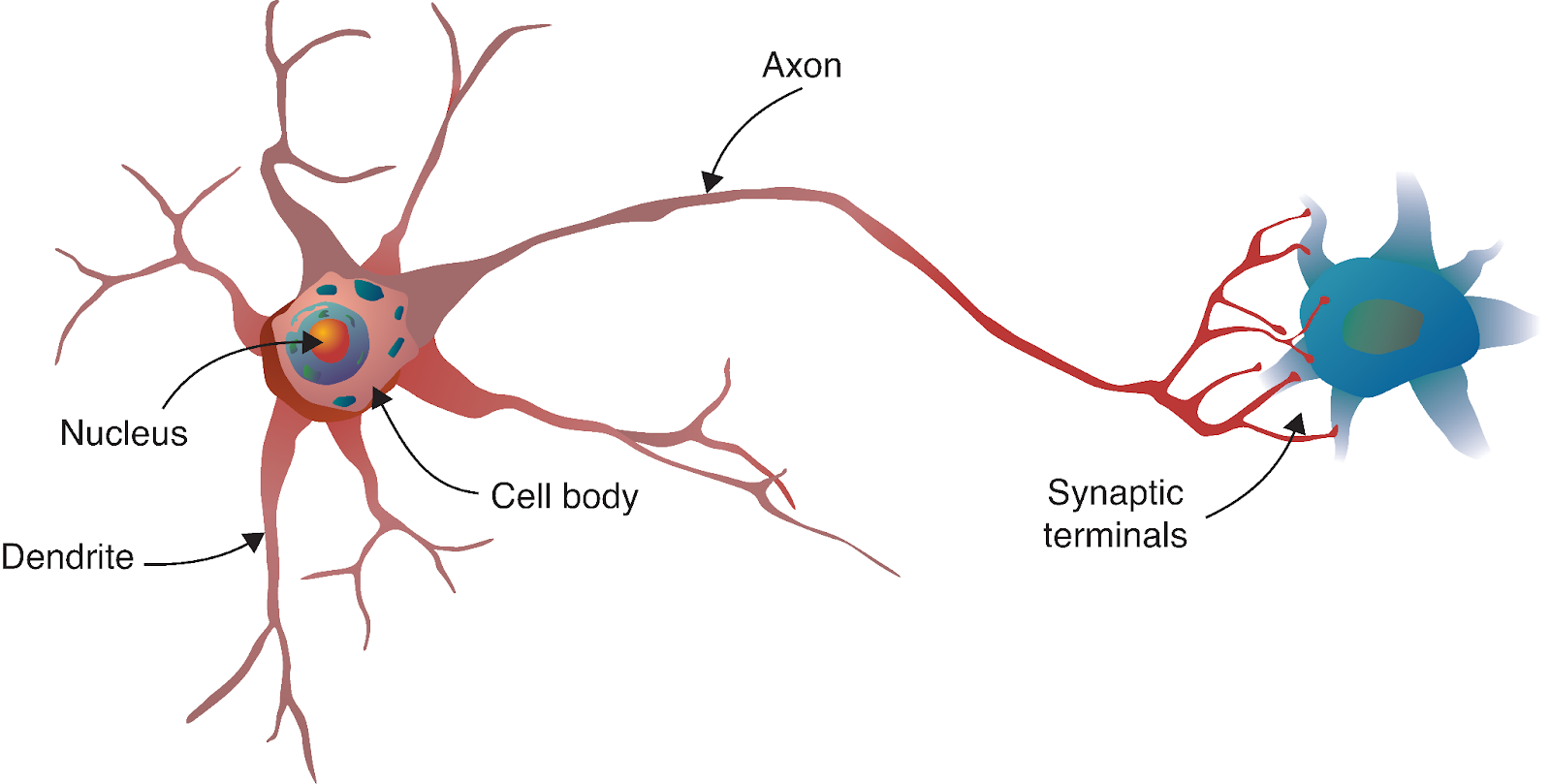
The neural network’s journey begins with a fascinating parallel to biology. Just as the human brain consists of billions of interconnected neurons, artificial neural networks are built from mathematical models inspired by these biological cells.

Source: Deep Learning - Visual Approach

A biological neuron receives signals from other neurons through dendrites, processes these signals in its cell body, and then transmits the result through the axon to other neurons. In our computational model, we mirror this process with:

• Inputs: The signals coming into the neuron (like dendrites receiving signals).
• Weights: The importance assigned to each input (analogous to the strength of synaptic connections).
• Bias: An additional parameter that helps the neuron activate or remain dormant regardless of inputs.
• Activation function: Determines whether and how strongly the neuron “fires” based on its inputs (similar to the cell body deciding whether to generate an action potential).
• Output: The signal sent to the next layer (like the axon transmitting to other neurons).

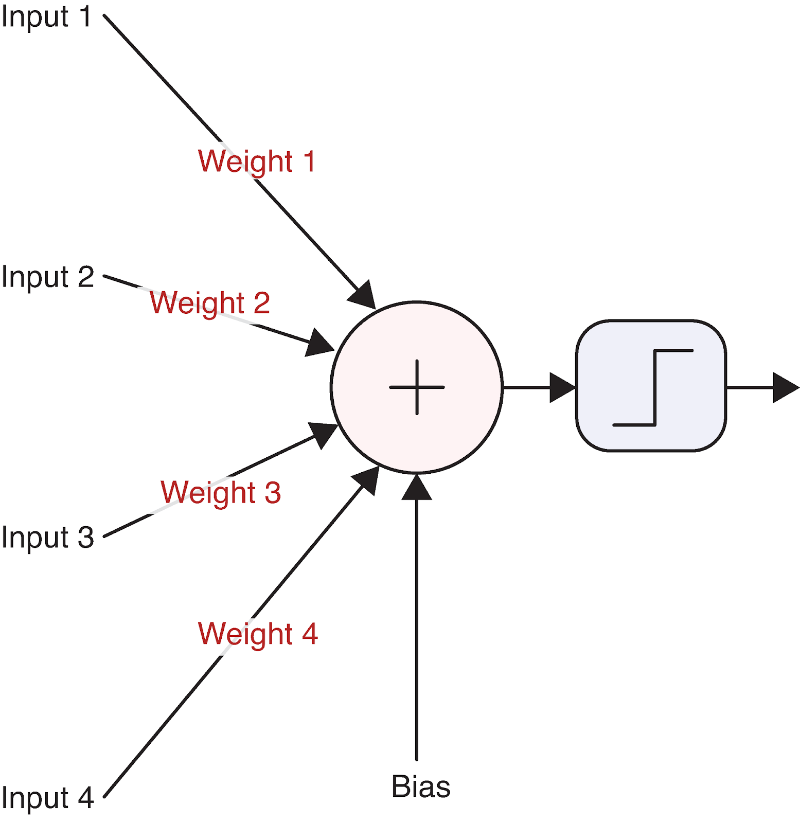
Let’s visualize a single neuron to make this concrete:

Source: Deep Learning - Visual Approach

This simple computational unit forms the foundation of even the most complex neural networks. But how exactly does a neuron transform its inputs into an output? This is where the math comes in.

Mathematical foundation of a single neuron

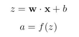
The operation of a neuron can be described with a straightforward equation:

Breaking this down:

• x is our input vector [x_1, x_2, x_3, …]
• w is our weight vector [w_1, w_2, …, w_n]
• b is the bias (a single scalar value)
• z is the weighted sum plus bias (often called the “pre-activation” or “logit”)
• f is the activation function
• a is the final output of the neuron

Let’s work through a concrete example with real numbers. Say we have a neuron with three inputs:

Inputs: x = [2, 5, -1]
Weights: w = [0.5, -1, 2]
Bias: b = 0.5

First, we calculate the weighted sum plus bias:

Next, we apply an activation function. Let’s use the popular ReLU (Rectified Linear Unit) function, which is defined as:

With a negative pre-activation value, our ReLU neuron outputs 0, meaning it doesn’t “fire” for this particular input.

The activation function is crucial because it introduces non-linearity into the network. Without it, neural networks would be limited to learning only linear relationships, regardless of how many layers they have. Common activation functions include:

• Sigmoid: — Outputs between 0 and 1, useful for binary classification
• ReLU: — Simple, efficient, and helps with the vanishing gradient problem
• Tanh:  — Outputs between -1 and 1, often used in hidden layers

Each activation function has its strengths and use cases, which we’ll explore more when implementing our neural network.

From neurons to layers

Individual neurons are powerful, but the true strength of neural networks emerges when neurons are organized into layers. A layer is simply a collection of neurons that process inputs in parallel. There are typically three types of layers in a neural network:

1. Input layer: Receives the raw data and passes it to the next layer
2. Hidden layers: Process information from previous layers
3. Output layer: Produces the final prediction or classification

When we have multiple neurons in a layer, each receiving the same inputs but with different weights and biases, we can efficiently represent this with matrix operations. Let’s see how this works.

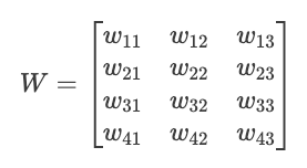
Imagine we have a layer with 3 input values and 4 neurons. Each neuron has its own set of weights and bias:

Inputs: x = [x₁, x₂, x₃]
Weights for neuron 1: w₁ = [w₁₁, w₁₂, w₁₃]
Weights for neuron 2: w₂ = [w₂₁, w₂₂, w₂₃]
Weights for neuron 3: w₃ = [w₃₁, w₃₂, w₃₃]
Weights for neuron 4: w₄ = [w₄₁, w₄₂, w₄₃]
Biases: b = [b₁, b₂, b₃, b₄]

We can organize these weights into a matrix W:

Now we can compute all neuron pre-activations at once with a single matrix multiplication:

Where:

• X is our input vector [x₁, x₂, x₃]
• W^T is the transpose of our weight matrix
• B is our bias vector [b₁, b₂, b₃, b₄]
• Z is the resulting vector of pre-activations [z₁, z₂, z₃, z₄]

Then we apply the activation function element-wise to get our final outputs:

This matrix representation is not just mathematical elegance; it’s also computational efficiency. Modern hardware (especially GPUs) is optimized for matrix operations, making this approach much faster than calculating each neuron’s output individually.

The ability to stack these layers — with the output of one layer becoming the input of the next — is what gives neural networks their remarkable capacity to learn complex patterns. As we connect these building blocks, we’re ready to explore how forward propagation works across an entire neural network.

Forward Propagation Through a Complete Network

Now that we understand individual neurons and layers, let’s step back and see how forward propagation works through an entire neural network. This is where the real power of deep learning emerges.

Multi-layer networks: the complete picture

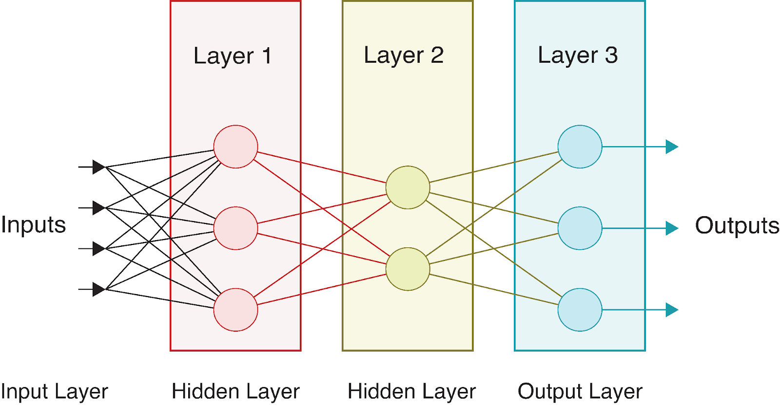
A full neural network consists of an input layer, one or more hidden layers, and an output layer. The term “deep” in deep learning refers to networks with multiple hidden layers. Each layer transforms the data in increasingly abstract ways, allowing the network to learn complex representations.

Let’s consider a simple neural network with:

• An input layer with 4 features
• Two hidden layers with 3 and 2 neurons, respectively
• An output layer with 3 neurons (perhaps for multi-class classification)

Visually, this network looks like:

As data flows through this network, we perform a series of calculations at each layer. If we denote:

• Input vector as X = [x_1, x_2, x_3, x_4]
• Weight matrices as (for the hidden layer) and (for the output layer)
• Bias vectors as and
• Activation functions as f1 (for the hidden layer) and f2 (for the output layer)

We can express the forward propagation through this entire network as:

1. Calculate hidden layer pre-activations: 

2. Apply activation function to get hidden layer outputs: 

3. Calculate output layer pre-activations: 

4. Apply activation function to get final outputs:

The final output A^[2] represents the network’s prediction. For classification problems, this might be probabilities for each class; for regression, it might be the predicted values.

Different layers often use different activation functions. For instance, hidden layers commonly use ReLU, while output layers might use:

• Sigmoid for binary classification
• Softmax for multi-class classification
• Linear (no activation) for regression

The beauty of this multi-layer structure is that each layer can learn to represent different aspects of the data. Early layers typically detect simple features, while deeper layers combine these into more complex patterns. This hierarchical learning is what makes neural networks so powerful for complex tasks like image and speech recognition.

Forward propagation algorithm

Let’s formalize the forward propagation process into an algorithm. For a neural network with L layers, forward propagation follows these steps:

# Pseudocode for forward propagation
def forward_propagation(X, parameters):
   """
   X: Input data (batch_size, n_features)
   parameters: Dictionary containing weights and biases for each layer
   Returns: The final output and all intermediate activations
   """
   # Store all activations for later use (e.g., in backpropagation)
   activations = {'A0': X}  # A0 is the input
  
   # Loop through L-1 layers (excluding the output layer)
   for l in range(1, L):
       # Get previous activation
       A_prev = activations[f'A{l-1}']
      
       # Get weights and biases for current layer
       W = parameters[f'W{l}']
       b = parameters[f'b{l}']
      
       # Compute pre-activation
       Z = np.dot(A_prev, W.T) + b
      
       # Apply activation function (e.g., ReLU for hidden layers)
       A = relu(Z)
      
       # Store values for later use
       activations[f'Z{l}'] = Z
       activations[f'A{l}'] = A
  
   # Compute output layer (layer L)
   A_prev = activations[f'A{L-1}']
   W = parameters[f'W{L}']
   b = parameters[f'b{L}']
  
   # Compute pre-activation for output layer
   Z = np.dot(A_prev, W.T) + b
  
   # Apply output activation function (depends on the task)
   if task == 'binary_classification':
       A = sigmoid(Z)
   elif task == 'multiclass_classification':
       A = softmax(Z)
   elif task == 'regression':
       A = Z  # Linear activation
  
   # Store output layer values
   activations[f'Z{L}'] = Z
   activations[f'A{L}'] = A
  
   return A, activations

This algorithm highlights several important aspects of forward propagation:

1. Sequential processing: Information flows strictly forward, layer by layer.
2. Activation storage: We store not just the final output but all intermediate activations, which will be crucial for training the network using backpropagation.
3. Task-specific output: The activation function for the output layer is chosen based on the specific problem (classification vs. regression).

The forward propagation algorithm is remarkably simple, yet it allows neural networks to approximate incredibly complex functions. When combined with proper training through backpropagation, this simple process enables the network to learn from data and make increasingly accurate predictions.

Let’s trace through a specific example to further solidify our understanding. Consider input X = [0.5, -0.2, 0.1] going through our example network with:

• Hidden layer weights W^[1] (4×3 matrix) and biases b^[1] (vector of 4 values)
• Output layer weights W^[2] (2×4 matrix) and biases b^[2] (vector of 2 values)

For simplicity, let’s say all weights are 0.1 and all biases are 0:

X = [0.5, -0.2, 0.1]
W[1] = [[0.1, 0.1, 0.1], [0.1, 0.1, 0.1], [0.1, 0.1, 0.1], [0.1, 0.1, 0.1]]
b[1] = [0, 0, 0, 0]
W[2] = [[0.1, 0.1, 0.1, 0.1], [0.1, 0.1, 0.1, 0.1]]
b[2] = [0, 0]

Following our algorithm:

• First step:

• Second step with ReLU: 

• Third step:

• Fourth step with using sigmoid: 

This gives us our final prediction. In a binary classification context, these values near 0.5 would indicate uncertainty between the two classes.

In the next section, we’ll implement forward propagation in Python to see these calculations in action.

Implementing Forward Propagation in Python

Now that we understand the theory behind forward propagation, let’s put it into practice by implementing it in Python. We’ll start with a “from scratch” implementation using only NumPy, then see how modern deep learning frameworks simplify this process.

Building from scratch with NumPy

NumPy provides efficient array operations that allow us to implement the matrix calculations we’ve discussed. Let’s build a simple neural network class that performs forward propagation through multiple layers.

First, we’ll need to import the necessary libraries:

import numpy as np
import matplotlib.pyplot as plt

# For reproducibility
np.random.seed(42)

Now, let’s define activation functions that we’ll use in our network:

def relu(Z):
   """ReLU activation function: max(0, Z)"""
   return np.maximum(0, Z)

def sigmoid(Z):
   """Sigmoid activation function: 1/(1 + e^(-Z))"""
   return 1 / (1 + np.exp(-Z))

def softmax(Z):
   """Softmax activation function for multi-class classification"""
   # Subtract max for numerical stability (prevents overflow)
   exp_Z = np.exp(Z - np.max(Z, axis=1, keepdims=True))
   return exp_Z / np.sum(exp_Z, axis=1, keepdims=True)

Next, let’s create a class for our neural network:

class NeuralNetwork:
   def __init__(self, layer_dims, activations):
       """
       Initialize a neural network with specified layer dimensions and activations
      
       Parameters:
       - layer_dims: List of integers representing the number of neurons in each layer
                    (including input and output layers)
       - activations: List of activation functions for each layer (excluding input layer)
       """
       self.L = len(layer_dims) - 1  # Number of layers (excluding input layer)
       self.layer_dims = layer_dims
       self.activations = activations
       self.parameters = {}
      
       # Initialize parameters (weights and biases)
       self.initialize_parameters()
  
   def initialize_parameters(self):
       """Initialize weights and biases with small random values"""
       for l in range(1, self.L + 1):
           # He initialization for weights - helps with training deep networks
           self.parameters[f'W{l}'] = np.random.randn(self.layer_dims[l], self.layer_dims[l-1]) * np.sqrt(2 / self.layer_dims[l-1])
           self.parameters[f'b{l}'] = np.zeros((self.layer_dims[l], 1))
  
   def forward_propagation(self, X):
       """
       Perform forward propagation through the network
      
       Parameters:
       - X: Input data (n_features, batch_size)
      
       Returns:
       - AL: Output of the network
       - caches: Dictionary containing all activations and pre-activations
       """
       caches = {}
       A = X  # Input layer activation
       caches['A0'] = X
      
       # Process through L-1 layers (excluding output layer)
       for l in range(1, self.L):
           A_prev = A
          
           # Get weights and biases for current layer
           W = self.parameters[f'W{l}']
           b = self.parameters[f'b{l}']
          
           # Forward propagation for current layer
           Z = np.dot(W, A_prev) + b
          
           # Apply activation function
           activation_function = self.activations[l-1]
           if activation_function == "relu":
               A = relu(Z)
           elif activation_function == "sigmoid":
               A = sigmoid(Z)
          
           # Store values for backpropagation
           caches[f'Z{l}'] = Z
           caches[f'A{l}'] = A
      
       # Output layer
       W = self.parameters[f'W{self.L}']
       b = self.parameters[f'b{self.L}']
       Z = np.dot(W, A) + b
      
       # Apply output activation function
       activation_function = self.activations[self.L-1]
       if activation_function == "sigmoid":
           AL = sigmoid(Z)
       elif activation_function == "softmax":
           AL = softmax(Z)
       elif activation_function == "linear":
           AL = Z  # No activation for regression
      
       # Store output layer values
       caches[f'Z{self.L}'] = Z
       caches[f'A{self.L}'] = AL
      
       return AL, caches

The NeuralNetwork class we've implemented above provides a complete framework for creating and using a neural network with customizable architecture. Let's break down its key components:

1. Initialization: The network is configured with specified layer dimensions and activation functions. It automatically initializes weights and biases using the He initialization method for better training performance.
2. Forward propagation: The forward_propagation method we just implemented is the heart of the neural network's prediction capability. It:

• Takes input data and passes it through each layer
• Applies the appropriate activation function at each layer
• Stores intermediate values in caches for later use in backpropagation
• Returns both the final output and all cached values

3. Activation functions: The network supports multiple activation functions, including ReLU, sigmoid, and softmax, allowing it to handle different types of problems (regression or classification).

4. Flexible architecture: The implementation allows for networks of arbitrary depth and width, making it suitable for a wide range of machine learning tasks.

This implementation follows the standard neural network design pattern where data flows forward through the network, with each layer transforming the data before passing it to the next layer.

Now let’s test our implementation with a small example network:

# Create a sample network
# Input layer: 3 features
# Hidden layer 1: 4 neurons with ReLU activation
# Output layer: 2 neurons with sigmoid activation (binary classification)
layer_dims = [3, 4, 2]
activations = ["relu", "sigmoid"]
nn = NeuralNetwork(layer_dims, activations)

# Create sample input data - 3 features for 5 examples
X = np.random.randn(3, 5)

# Perform forward propagation
output, caches = nn.forward_propagation(X)

print(f"Input shape: {X.shape}")
print(f"Output shape: {output.shape}")
print(f"Output values:\n{output}")

Output:

Input shape: (3, 5)
Output shape: (2, 5)
Output values:
[[0.00386784 0.54343014 0.39661893 0.5        0.51056934]
[0.11877049 0.32541093 0.44840699 0.5        0.45586633]]

Let’s also visualize how the data transforms as it flows through the network:

def visualize_activations(caches, example_idx=0):
   """Visualize the activations for a single example through the network"""
   plt.figure(figsize=(15, 6))
  
   # Plot input
   plt.subplot(1, 3, 1)
   plt.bar(range(caches['A0'].shape[0]), caches['A0'][:, example_idx])
   plt.title('Input Layer')
   plt.xlabel('Feature')
   plt.ylabel('Value')
  
   # Plot hidden layer activation
   plt.subplot(1, 3, 2)
   plt.bar(range(caches['A1'].shape[0]), caches['A1'][:, example_idx])
   plt.title('Hidden Layer (ReLU Activation)')
   plt.xlabel('Neuron')
   plt.ylabel('Activation')
  
   # Plot output layer
   plt.subplot(1, 3, 3)
   plt.bar(range(caches['A2'].shape[0]), caches['A2'][:, example_idx])
   plt.title('Output Layer (Sigmoid Activation)')
   plt.xlabel('Neuron')
   plt.ylabel('Activation')
  
   plt.tight_layout()
   plt.show()

# Visualize the first example
visualize_activations(caches)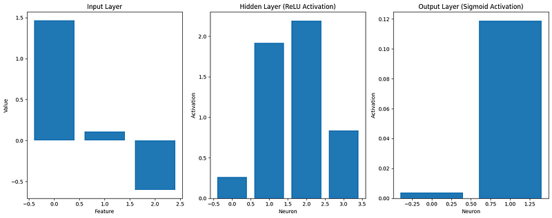

This visualization helps us understand how the input data is transformed as it propagates through the network. We can see that:

1. The input features might have positive or negative values
2. After ReLU activation in the hidden layer, all activations are non-negative
3. The sigmoid activation in the output layer constrains values between 0 and 1

Our “from scratch” implementation demonstrates the core principles of forward propagation, but modern deep learning frameworks provide more efficient and flexible tools for building neural networks.

Using deep learning frameworks

Now, let’s implement the same neural network using popular deep learning frameworks: TensorFlow and PyTorch. These frameworks optimize performance and provide higher-level abstractions, making it easier to build complex models.

First, let’s look at TensorFlow/Keras implementation:

import tensorflow as tf
from tensorflow.keras.models import Sequential
from tensorflow.keras.layers import Dense, Input

# For reproducibility
tf.random.set_seed(42)

# Create the same network architecture
tf_model = Sequential([
   Input(shape=(3,)),  # Input layer with 3 features
   Dense(4, activation='relu'),  # Hidden layer with 4 neurons
   Dense(2, activation='sigmoid')  # Output layer with 2 neurons
])

tf_model.summary()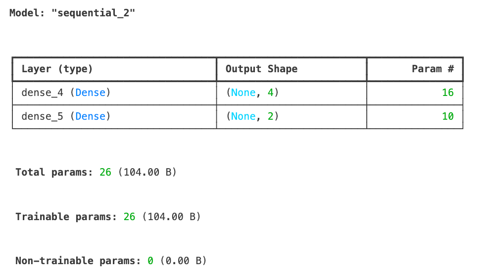

# Sample input data with the shape expected by Keras
X_tf = np.random.randn(5, 3)  # 5 examples, 3 features

# Forward propagation in TensorFlow
tf_output = tf_model.predict(X_tf)

print(f"TensorFlow output shape: {tf_output.shape}")
print(f"TensorFlow output values:\n{tf_output}")

TensorFlow output shape: (5, 2)
TensorFlow output values:
[[0.6855308  0.7139542 ]
[0.4952355  0.5231934 ]
[0.50174904 0.5198488 ]
[0.44331825 0.6860926 ]
[0.6624589  0.5385444 ]]

We’ve just implemented our neural network using TensorFlow/Keras and successfully performed forward propagation on some sample data. The model summary shows our architecture with an input layer accepting 3 features, a hidden layer with 4 neurons using ReLU activation, and an output layer with 2 neurons using sigmoid activation. In total, the model has 26 trainable parameters.

The forward propagation results show the output shape (5, 2) corresponding to our 5 input examples, each producing 2 output values. These outputs are constrained between 0 and 1 due to the sigmoid activation function in the output layer.

Next, let’s see how we can implement the same neural network architecture using PyTorch, another popular deep learning framework, to compare the approaches.

import torch
import torch.nn as nn

# For reproducibility
torch.manual_seed(42)

# Create a network in PyTorch
class PyTorchNN(nn.Module):
   def __init__(self):
       super(PyTorchNN, self).__init__()
       self.hidden = nn.Linear(3, 4)  # 3 inputs, 4 hidden neurons
       self.relu = nn.ReLU()
       self.output = nn.Linear(4, 2)  # 4 inputs from hidden, 2 outputs
       self.sigmoid = nn.Sigmoid()
  
   def forward(self, x):
       x = self.relu(self.hidden(x))
       x = self.sigmoid(self.output(x))
       return x

# Instantiate the model
torch_model = PyTorchNN()

# Print model structure
print(torch_model)

Output:

PyTorchNN(
 (hidden): Linear(in_features=3, out_features=4, bias=True)
 (relu): ReLU()
 (output): Linear(in_features=4, out_features=2, bias=True)
 (sigmoid): Sigmoid()
)

```python
# Sample input data
X_torch = torch.randn(5, 3)  # 5 examples, 3 features

# Forward propagation in PyTorch
torch_output = torch_model(X_torch)

print(f"PyTorch output shape: {torch_output.shape}")
print(f"PyTorch output values:\n{torch_output}")

Output:

PyTorch output shape: torch.Size([5, 2])
PyTorch output values:
tensor([[0.4516, 0.4116],
       [0.4289, 0.4267],
       [0.4278, 0.4172],
       [0.3771, 0.4321],
       [0.5769, 0.3328]], grad_fn=<SigmoidBackward0>)

Let’s compare our implementations:

# Compare dimensions and structure of outputs
print("\nComparison of implementations:")
print(f"NumPy output shape: {output.shape}")
print(f"TensorFlow output shape: {tf_output.shape}")
print(f"PyTorch output shape: {torch_output.shape}")

Output:

Comparison of implementations:
NumPy output shape: (2, 5)
TensorFlow output shape: (5, 2)
PyTorch output shape: torch.Size([5, 2])

The key differences between our implementations:

1. Structure and readability:

• NumPy: Explicit implementation of each step gives complete control and transparency
• TensorFlow/Keras: High-level abstractions hide implementation details but make code simpler
• PyTorch: Object-oriented approach with explicit forward method

2. Performance:

• TensorFlow and PyTorch optimize operations for GPU acceleration
• Both frameworks implement efficient gradient computation for training
• Frameworks optimize memory usage for large networks

3. Extensibility:

• Frameworks provide pre-built components (layers, optimizers, etc.)
• Built-in tools for saving/loading models, visualization, and deployment
• Extensive community support and documentation

For simple networks, our NumPy implementation works fine, but as complexity increases, deep learning frameworks become essential. They handle low-level optimizations and provide tools for the entire machine learning workflow, from development to deployment. To learn more about these frameworks, check out our separate guides:

• PyTorch Tutorial: Building a Simple Neural Network From Scratch
• TensorFlow Tutorial For Beginners 

In the next section, we’ll build a complete working example that applies forward propagation to a real-world problem.

Forward Propagation Example

Now that we’ve implemented forward propagation both from scratch and using popular frameworks, let’s see it in action on a real-world problem. We’ll build a complete example and explore how to optimize the process for better performance.

Complete working example

Let’s apply our understanding to a classic machine learning problem: handwritten digit recognition using the MNIST dataset. This dataset contains 70,000 images of handwritten digits (0–9), each 28x28 pixels in size.

First, let’s load and prepare the data:

from tensorflow.keras.datasets import mnist
import numpy as np
import matplotlib.pyplot as plt

# Load MNIST dataset
(X_train, y_train), (X_test, y_test) = mnist.load_data()

# Normalize pixel values to range [0, 1]
X_train = X_train / 255.0
X_test = X_test / 255.0

# Reshape images to vectors (flatten 28x28 to 784)
X_train_flat = X_train.reshape(X_train.shape[0], -1).T  # Shape: (784, 60000)
X_test_flat = X_test.reshape(X_test.shape[0], -1).T     # Shape: (784, 10000)

# Convert labels to one-hot encoding
def one_hot_encode(y, num_classes=10):
   one_hot = np.zeros((num_classes, y.size))
   one_hot[y, np.arange(y.size)] = 1
   return one_hot

y_train_one_hot = one_hot_encode(y_train)  # Shape: (10, 60000)
y_test_one_hot = one_hot_encode(y_test)    # Shape: (10, 10000)

# Display sample images
plt.figure(figsize=(10, 5))
for i in range(5):
   plt.subplot(1, 5, i+1)
   plt.imshow(X_train[i], cmap='gray')
   plt.title(f"Label: {y_train[i]}")
   plt.axis('off')
plt.tight_layout()
plt.show()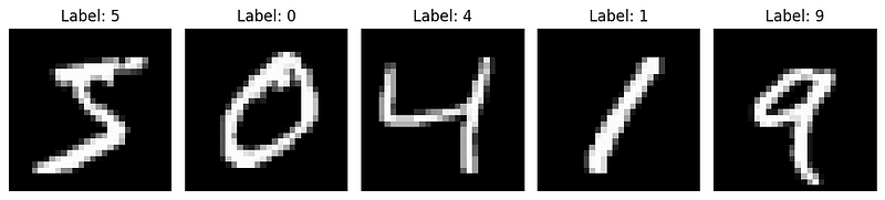

Now, let’s build a neural network for this task using our NumPy implementation. We’ll create a network with:

• Input layer: 784 neurons (28x28 pixels)
• Hidden layer: 128 neurons with ReLU activation
• Output layer: 10 neurons with softmax activation (for 10 digits)

# Define our network architecture
layer_dims = [784, 128, 10]
activations = ["relu", "softmax"]
nn = NeuralNetwork(layer_dims, activations)

# Take a small batch for demonstration
batch_size = 64
batch_indices = np.random.choice(X_train_flat.shape[1], batch_size, replace=False)
X_batch = X_train_flat[:, batch_indices]
y_batch = y_train_one_hot[:, batch_indices]

# Perform forward propagation
output, caches = nn.forward_propagation(X_batch)

# Compute accuracy
predictions = np.argmax(output, axis=0)
true_labels = np.argmax(y_batch, axis=0)
accuracy = np.mean(predictions == true_labels)

print(f"Batch accuracy: {accuracy:.4f}")

Out: Batch accuracy: 0.0781

We’ve got 7% accuracy, which is worse than even a random guessing model. But that’s expected since we are only performing forward propagation — there is no learning involved.

Now, let’s visualize how the network processes a single image through each layer:

def visualize_network_processing(nn, image, label, caches):
   """Visualize network processing for a single image"""
   plt.figure(figsize=(15, 10))
  
   # Plot original image
   plt.subplot(2, 3, 1)
   plt.imshow(image.reshape(28, 28), cmap='gray')
   plt.title(f"Input Image (Digit: {label})")
   plt.axis('off')
  
   # Plot flattened input (first 100 values)
   plt.subplot(2, 3, 2)
   plt.bar(range(100), image.flatten()[:100])
   plt.title("Input Layer (first 100 pixels)")
   plt.xlabel("Pixel Index")
   plt.ylabel("Pixel Value")
  
   # Plot hidden layer activations (first 50 neurons)
   plt.subplot(2, 3, 3)
   hidden_activations = caches['A1'][:50, 0]
   plt.bar(range(len(hidden_activations)), hidden_activations)
   plt.title("Hidden Layer Activations (first 50 neurons)")
   plt.xlabel("Neuron Index")
   plt.ylabel("Activation")
  
   # Plot output layer activations
   plt.subplot(2, 3, 4)
   output_activations = caches['A2'][:, 0]
   plt.bar(range(10), output_activations)
   plt.xticks(range(10))
   plt.title("Output Layer Activations (Softmax)")
   plt.xlabel("Digit Class")
   plt.ylabel("Probability")
  
   # Plot prediction vs actual
   plt.subplot(2, 3, 5)
   prediction = np.argmax(output_activations)
   plt.bar(['Actual', 'Predicted'], [label, prediction], color=['blue', 'orange'])
   plt.title(f"Prediction: {prediction}, Actual: {label}")
   plt.ylabel("Digit")
  
   plt.tight_layout()
   plt.show()

# Visualize forward propagation for the first image in our batch
image_idx = 0
image = X_batch[:, image_idx].reshape(784, 1)
label = true_labels[image_idx]

visualize_network_processing(nn, image, label, caches)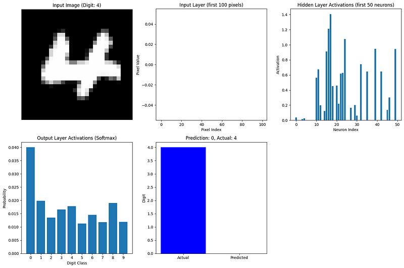

This visualization shows how information flows through our network:

1. Input layer: The flattened image pixels (values between 0 and 1)
2. Hidden layer: The ReLU-activated neurons capture different features of the digit
3. Output layer: The softmax activation gives a probability distribution over the 10 possible digits

The most active output neuron corresponds to the network’s prediction. Even with random weights (since we haven’t trained the network yet), we can see how forward propagation transforms the input data into a prediction.

For a more complete example, we would train this network using backpropagation to adjust the weights and biases, improving the predictions over time. However, even without training, this example demonstrates the forward propagation process on real data.

Optimizing forward propagation

As neural networks grow larger and datasets become more massive, optimizing forward propagation becomes crucial. Here are key strategies for making forward propagation more efficient:

1. Batch processing

Rather than processing one example at a time, we compute forward propagation on batches of examples simultaneously. This leverages the parallel processing capabilities of modern hardware.

2. Vectorization

Using matrix operations instead of loops dramatically speeds up computation. This is why our implementation used NumPy’s array operations.

3. Memory management

For large networks, we need to be careful about memory usage. Techniques include:

• Reusing memory for intermediate activations.
• Computing activations layer by layer without storing all intermediates.
• Using lower precision representations (e.g., 16-bit floats instead of 32-bit).

4. GPU acceleration

Graphics Processing Units excel at matrix operations. Modern frameworks can seamlessly move computation to GPUs for significant speedups:

# TensorFlow example of GPU acceleration
import tensorflow as tf

# Check for available GPUs
print("GPUs Available:", tf.config.list_physical_devices('GPU'))

# TensorFlow automatically uses available GPUs
with tf.device('/GPU:0'):  # Explicitly specify GPU if multiple are available
   # Computation runs on GPU if available
   result = tf_model.predict(X_tf)

5. Specialized hardware

Beyond GPUs, hardware like Google’s Tensor Processing Units (TPUs) are specifically designed for neural network operations.

6. Algorithmic optimizations

Certain activation functions and network architectures are designed for computational efficiency:

• ReLU is faster to compute than sigmoid or tanh.
• Depthwise separable convolutions reduce computation compared to standard convolutions.
• Network pruning removes unnecessary connections, reducing computation.

7. Framework optimizations

Deep learning frameworks implement numerous low-level optimizations:

• Fused operations combine multiple steps into single-optimized kernels.
• Auto-tuned algorithms select the fastest implementation for specific hardware.
• JIT (Just-In-Time) compilation creates optimized code for specific network configurations.

As networks become deeper and wider, forward propagation optimization becomes increasingly important. Modern architectures like ResNets, Transformers, and EfficientNets incorporate design choices specifically to make forward propagation more efficient while maintaining or improving model accuracy.

In the next section, we’ll explore how forward propagation connects to backward propagation (backpropagation), completing the picture of how neural networks learn.

The Relationship with Backpropagation

We’ve now explored forward propagation thoroughly, but this is only half of the story when it comes to neural networks. Let’s briefly examine how forward propagation connects with backpropagation, the algorithm that enables neural networks to learn.

Connecting forward and backward propagation

Forward propagation and backpropagation work as complementary processes in neural networks:

• Forward propagation takes inputs and produces predictions, moving from left to right through the network.
• Backpropagation takes errors and produces weight updates, moving from right to left through the network.

These two processes are inseparable in the learning process. Backpropagation cannot happen without first performing forward propagation, as it needs:

1. The activations from each layer (which we stored in our caches).
2. The final prediction to compare against the true label.
3. The network architecture and weights used during forward propagation.

Think of forward propagation as a neural network making its best guess, given its current understanding, while backpropagation is how it refines that understanding based on its mistakes.

The learning loop

The entire learning process follows a cyclical pattern:

1. Forward propagation: The network processes the input data and makes predictions.
2. Loss calculation: The predictions are compared to the actual targets to calculate error.
3. Backward propagation: The error is propagated backward through the network to determine how each weight contributed to the error.
4. Weight update: The weights are adjusted to reduce the error.
5. Repeat: The process continues with new data until the network performs well.

What makes this process powerful is that forward propagation provides the context needed for backpropagation. During forward propagation, the network not only makes predictions but also keeps track of all the intermediate values and decisions. Backpropagation then uses this information to make targeted adjustments.

The beauty of this system is that complex learning emerges from these two relatively simple processes working together. Forward propagation is straightforward — it’s just matrix multiplications and activation functions applied sequentially. Backpropagation is more complex but follows directly from calculus principles.

Together, they enable neural networks to learn virtually any pattern given enough data and computational resources. This learning capability has powered breakthroughs in computer vision, natural language processing, game playing, and countless other domains.

Understanding forward propagation thoroughly, as we’ve done in this article, provides the foundation needed to grasp the complete learning process in neural networks. If you’re interested in diving deeper into the learning aspect, our guide on backpropagation provides a detailed exploration of how networks learn from their mistakes.

Conclusion and Next Steps

Forward propagation is the foundational process that enables neural networks to transform inputs into predictions. As we’ve explored, it involves sequential matrix multiplications and activation functions that progressively transform data through the network’s layers. Understanding this process is crucial whether you’re implementing networks from scratch, using modern frameworks, or troubleshooting model performance. 

By mastering forward propagation, you’ve taken a significant step toward building and understanding deep learning models that can tackle complex problems across domains.

To continue your deep learning journey, explore DataCamp’s comprehensive resources: 

• Dive into the mathematics behind neural networks with Introduction to Deep Neural Networks
• Master the training process with Mastering Backpropagation
• Get hands-on experience building networks in PyTorch or R. 

For a structured learning path, the Deep Learning in Python track provides everything you need to become proficient in building and deploying neural networks for real-world applications.