Mean Shift Clustering: A Comprehensive Guide

Discover the mean shift clustering algorithm, its advantages, real-world applications, and step-by-step Python implementation. Compare it with K-means to understand key differences.

Sep 12, 2024 · 11 min read

Clustering is an unsupervised machine learning technique that identifies hidden structures in the data to help businesses make more informed decisions. Some of the most common clustering applications are image segmentation, customer segmentation, and social network analysis.

Based on whether the algorithm requires an input of a predetermined number of clusters or the distribution of data, clustering is of two types – parametric and non-parametric. In this post, we will cover one such non-parametric algorithm in detail–the mean shift clustering algorithm. We will discuss its underlying principles, explore its applications in different industries, and provide a Python implementation. Toward the end, we will compare it with the popular k-means clustering technique.

What is Mean Shift Clustering?

Mean shift clustering is used to identify clusters in datasets where the number of clusters is not known beforehand. It finds clusters by iteratively shifting data points toward the densest regions in the feature space. This makes it particularly useful for applications such as object recognition, where it can segment images based on pixel intensity and color, and also for tracking objects in video sequences.

As a mode-seeking algorithm, it labels the clusters by finding the modes, or peaks, in the data distribution. Essentially, it highlights the most dense areas. It does this by iteratively shifting the cluster centers toward regions of a higher data density. Here are the steps:

Initialization: Start by considering each data point as a potential candidate for the cluster center.
Density Estimation: For each data point, define a window around it, called the radius, and then compute the mean of those data points within this radius.
Shifting: Shift each point to this mean position. This step moves the point towards the region of higher density.
Convergence: Repeat steps 2 and 3 iteratively until convergence, i.e., when the shift is smaller than a predefined threshold. The insignificant change in shift implies that the points have stabilized around the local maxima of the density function.

At the end of this iterative process, data points cluster around the modes of the data distribution, forming the clusters. Mean shift is particularly flexible because it relies on the actual data distribution rather than assuming a predefined shape for clusters, which allows it to handle clusters of arbitrary shapes.

Why Use Mean Shift Clustering?

Mean shift clustering is a powerful tool for uncovering the underlying structure of data without making any assumptions about its parameters such as the number of clusters or their shape. Considering its density-based approach that focuses on regions of high data density, it is robust against outliers, thereby ensuring that noisy data has minimal impact on the clustering process. Such robustness makes it an apt fit for real-world datasets, which often contain irregularities and noise, and also for applications requiring adaptability and precision.

Some of the real-world scenarios where mean shift clustering works well are:

Image segmentation

The mean shift clustering algorithm can segment images into regions based on pixel intensity or color without requiring prior knowledge of the number of segments. This flexibility makes it highly effective for image segmentation tasks because the clusters generated using mean shift clustering can take any shape or size.

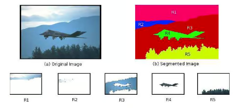
Image segmentation using mean shift clustering. Source: ResearchGate

Also, images that contain noise, particularly in low-light conditions, are difficult to segment. For such scenarios, the mean shift clustering algorithm provides more natural and accurate segmentation, which is essential in applications like medical imaging for detecting abnormal tissue types or in computer vision for reliable object detection.

Object tracking in video analysis

Following its advantages in image segmentation, mean shift clustering is frequently used in object tracking within video streams. Its ability to dynamically identify and follow objects as they move across frames makes it quite effective for real-time tracking applications.

Mean shift clustering in object tracking. Source: ResearchGate

By focusing on the density of pixels or features associated with the object, mean shift can effectively track objects of varying shapes and sizes, making it easily adapt to changes in movement and appearance.

Customer segmentation in marketing

For businesses, it is important to understand customer segments without assuming a fixed number of categories while also accounting for outlier behavior. mean shift clustering can analyze customer behavior, purchasing patterns, and demographic data to uncover natural groupings irrespective of the group size.

This helps create targeted marketing strategies and personalized experiences, ultimately enhancing customer engagement and retention.

How Does Mean Shift Clustering Work?

Let’s start with a function to estimate the density of data points in a window and understand how this algorithm works.

Kernel density estimation (KDE)

It uses a probability density function of a random variable to identify areas of higher data density in each iteration. The formula for KDE is:

Where h is a bandwidth parameter, and the kernel is commonly a Gaussian. The kernel function k smooths the contribution of each data point, ensuring that points closer to x have a higher influence on the density estimate.

Choosing the right bandwidth

The bandwidth parameter h determines the size of the neighborhood around each data point, directly influencing the clustering results. Here are methods to select the bandwidth:

Scott’s rule

Scott’s rule is a heuristic approach that provides a rule of thumb for bandwidth selection. It balances bias and variance in the density estimate, making it a good starting point for many applications.

where:

n is the number of data points.
d is the number of dimensions in the dataset.

Silverman’s rule

Similar to Scott’s rule, Silverman’s rule offers another heuristic approach for bandwidth selection particularly useful for unimodal distributions.

Cross-validation

By evaluating the performance of different bandwidth values on the holdout datasets, we can choose the best bandwidth value that minimizes error and yields the best clustering results.

Split the data into training and validation sets.
Apply mean shift clustering with different bandwidth values on the training set.
Evaluate the performance corresponding to each bandwidth on the validation set.
Select the bandwidth that minimizes the error.

Expert knowledge

Expert knowledge can provide valuable insights on selecting the appropriate bandwidth, especially in specific applications, such as image processing. An expert might understand the typical scale of features within the image to choose the optimal bandwidth range and then fine-tune this range through empirical testing.

Adaptive bandwidth

Adaptive bandwidth is useful for datasets with varying densities. It applies different bandwidths for different regions of the data. It starts with a global bandwidth estimate and then adjusts it locally based on the density of data points in that region.

Mean shift vector

The mean shift vector represents the magnitude and direction of the movement required to shift the cluster center estimate from lower-density areas to higher-density regions.

For a data point xi, the mean shift vector m(xi) is calculated as:

where N(xi) denotes the neighborhood around xi defined by the bandwidth.

Convergence

The mean shift clustering algorithm converges when cluster centers no longer move beyond a specified threshold and when the algorithm has identified the modes of the density function, around which clusters are formed. The algorithm continues iterating through the following steps until convergence:

Calculate the mean shift vector for each data point.
Shift the data point towards the mean of its neighborhood.
Check for convergence by determining if the shifts are smaller than a predefined threshold.

Convergence indicates that data points have stabilized around the local maxima of the density function, which then serve as the cluster centers.

Become a ML Scientist

Master Python skills to become a machine learning scientist

Start Learning for Free

Implementation of Mean Shift Clustering in Python

It’s time to explore the steps involved in using mean shift clustering. We’ll use the MeanShift class from the popular sci-kit-learn library, which is available out of the box to apply this algorithm to datasets.

Basic mean shift clustering

Let’s begin by importing the required libraries for the implementation.

from sklearn.cluster import MeanShift, estimate_bandwidth
from sklearn.datasets import make_blobs
import matplotlib.pyplot as plt

Next, we’ll generate a synthetic dataset of 500 samples using the make_blobs() function from scikit-learn’s datasets module. The dataset will have five centers, i.e., clusters, with a 0.7 cluster standard deviation.

# Create a sample dataset
X, _ = make_blobs(n_samples=500, centers=5, cluster_std=0.7, random_state=27)

Let’s estimate the bandwidth using the estimate_bandwidth() function.

# Estimate the bandwidth of the input data
bandwidth = estimate_bandwidth(X, quantile=0.2, n_samples=500)

Now, we’ll use this bandwidth number to initialize the MeanShift clustering object and fit it over the dataset we created earlier.

# Perform mean shift clustering
ms_model = MeanShift(bandwidth=bandwidth, bin_seeding=True)
ms_model.fit(X)
labels = ms_model.labels_
mean_shift_centers = ms_model.cluster_centers_

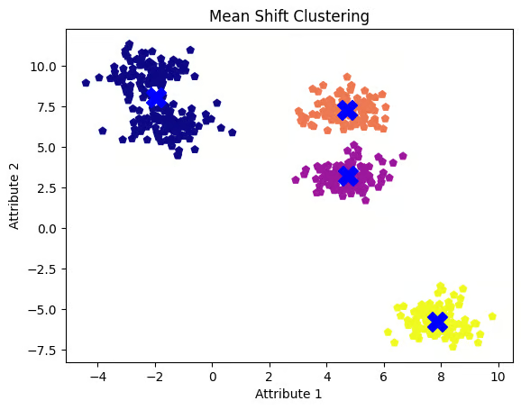
It’s time to visualize the mean shift cluster centers over our original dataset. Here, our five clusters are represented in different colors with mean shift centers represented by crosses.

# Plot the results
plt.scatter(X[:, 0], X[:, 1], c=labels, cmap='plasma', marker='p')
plt.scatter(mean_shift_centers[:, 0], mean_shift_centers[:, 1], s=250, c='blue', marker='X')
plt.title('mean shift clustering')
plt.xlabel('Attribute 1')
plt.ylabel('Attribute 2')
plt.show()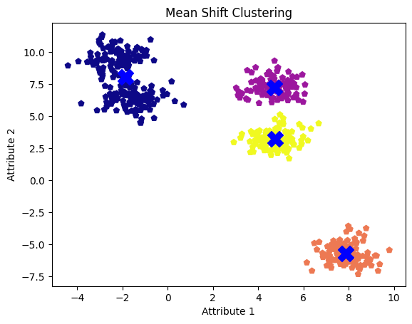

Mean shift clusters with default bandwidth value. Image by Author

Although we observe five blobs or clusters, the algorithm only identifies four by merging two adjacent clusters into one.

Tuning bandwidth parameter

The bandwidth parameter has a significant impact on clustering results. Let’s tune it to see if we can find the five clusters. We will test three different bandwidth values and visualize the resulting cluster centers for each.

# Try different bandwidth values
bandwidth_values = [0.1, 1.0, 2.0]

for bw in bandwidth_values:
    ms = MeanShift(bandwidth=bw, bin_seeding=True)
    ms.fit(X)
    labels = ms.labels_
    cluster_centers = ms.cluster_centers_
    print("Bandwidth Value:", bw)
    plt.scatter(X[:, 0], X[:, 1], c=labels, cmap='plasma', marker='p')
    plt.scatter(cluster_centers[:, 0], cluster_centers[:, 1], s=250, c='blue', marker='X')
    plt.title('mean shift clustering')
    plt.xlabel('Attribute 1')
    plt.ylabel('Attribute 2')
    plt.show()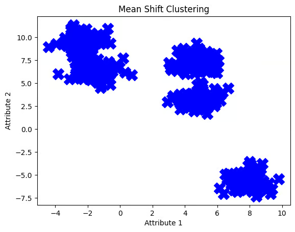

Mean shift clusters with 0.1 bandwidth value. Image by Author

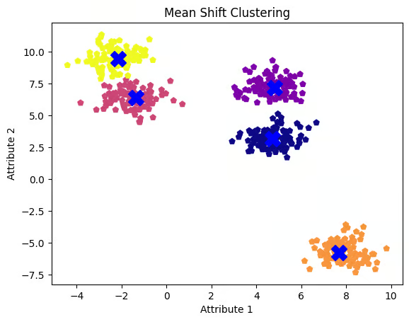
Mean shift clusters with 1.0 bandwidth value. Image by Author

Mean shift clusters with 2.0 bandwidth value. Image by Author

The bandwidth value of 0.1 seems to be too low, causing the algorithm to treat each data point as a separate cluster. On the other hand, a bandwidth value of 2.0 appears somewhat high, as it did not separate the two clusters in our first attempt. A bandwidth value of 1.0 proves to be the most optimal, clearly revealing all five clusters and their centers.

Let’s select this value and visualize the results once more.

ms = MeanShift(bandwidth=1.0, bin_seeding=True)
ms.fit(X)
labels = ms.labels_
cluster_centers = ms.cluster_centers_
plt.scatter(X[:, 0], X[:, 1], c=labels, cmap='plasma', marker='p')
plt.scatter(cluster_centers[:, 0], cluster_centers[:, 1], s=250, c='blue', marker='X')
plt.title('mean shift clustering')
plt.xlabel('Attribute 1')
plt.ylabel('Attribute 2')
plt.show()

Mean shift clusters with 1.0 bandwidth value

As observed, a smaller bandwidth tends to produce more clusters, while a larger bandwidth can lead to the merging of clusters.

Comparing mean shift with k-means

Let’s compare the results of mean shift and k-means clustering on the same dataset. First, import KMeans from sklearn’s cluster module. Next, we’ll set the number of clusters to three and fit the model to get the cluster centroids.

from sklearn.cluster import KMeans
# Perform k-means Clustering
kmeans = KMeans(n_clusters=3, random_state=0, n_init='auto')
kmeans.fit(X)
kmeans_labels = kmeans.labels_
kmeans_centers = kmeans.cluster_centers_

Now, let’s visualize the results to compare them with the mean shift clustering results.

plt.scatter(X[:, 0], X[:, 1], c=kmeans_labels, cmap='plasma', marker='p')
plt.scatter(kmeans_centers[:, 0], kmeans_centers[:, 1], s=250, c='red', marker='X')
plt.title('K-means Clustering')
plt.xlabel('Attribute 1')
plt.ylabel('Attribute 2')
plt.show()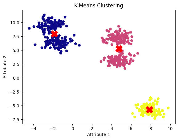

k-means clustering results. Image by Author

The drawback of the k-means clustering algorithm is that it requires specifying the number of clusters in advance, which can lead to merging adjacent clusters into one. However, a well-tuned mean shift clustering model successfully identified all five clusters and their centers.

Real-World Use Cases

In addition to object recognition in image processing, mean shift clustering is used in a number of real-world applications across multiple domains:

It supports gene expression analysis and protein structure prediction in bioinformatics.
Geospatial analysts leverage it for geographical clustering and anomaly detection in spatial data.
In medical imaging, it is used to detect tumors in MRI and CT scans, as well as for tissue classification.
The finance sector uses it for market segmentation and fraud detection.
Additionally, in natural language processing (NLP), it is applied to document clustering and sentiment analysis.

Conclusion

In this post, we learned how mean shift clustering adapts to varying cluster shapes and sizes, all without needing a predefined number of clusters.

With all the insights and practical implementation of this algorithm, you are all set to experiment with it in your projects. Python is the most popular programming language, and is well worth learning. You can refer to this Python Developer career track to take your Python programming skills to the next level. Also, check out our full Machine Learning Scientist with Python career track, and learn from experts.

Become an ML Scientist

Upskill in Python to become a machine learning scientist.

Start Learning for Free

Author

Vidhi Chugh

What is mean shift clustering?

How does mean shift clustering differ from k-means?

What are the real-world applications of mean shift clustering?

How do you select the bandwidth parameter in mean shift clustering?

What are the key steps in implementing mean shift clustering in Python?

Topics

Data Science

Python

blog

Classification vs Clustering in Machine Learning: A Comprehensive Guide

Explore the key differences between Classification and Clustering in machine learning. Understand algorithms, use cases, and which technique to use for your data science project.