Linear Discriminant Analysis: Beyond Dimension Reduction

Linear discriminant analysis (LDA) often gets overshadowed by a more popular algorithm, principal component analysis (PCA), when it comes to dimensionality reduction. However, LDA offers something unique that PCA cannot: it simultaneously reduces dimensions while optimizing for class separability.

This tutorial will introduce you to LDA, the mathematical intuition behind it, and real-world applications of the technique. Further, we will implement LDA on a dataset, comparing it with PCA, and analyse its advantages and disadvantages, aiming to provide everything you need to start applying LDA in your next project.

Introduction to Linear Discriminant Analysis (LDA)

LDA is a dimension reduction and classification technique under the assumption that different classes generate data based on different Gaussian distributions. 

LDA aims to find a linear combination of features that best separates these classes. It maximizes the ratio of between-class scatter to within-class scatter. In simpler terms, it tries to find directions in the feature space where different classes are far apart from each other (high between-class scatter) while points within the same class are close together (low within-class scatter). 

This dual objective makes LDA particularly effective for both dimensionality reduction and classification tasks.

Mathematics Behind the LDA

Understanding the mathematics behind LDA requires breaking down the algorithm into three key components: 

• within-class scatter, 
• between-class scatter, and
• optimization objective.

Within-class scatter matrix (Sw)

The within-class scatter matrix measures how scattered the data points are within each class. 

For each class i, we calculate the scatter matrix Si as:

Si = Σ(x - μi)(x - μi)T

Where x represents each data point in class i, and μi is the mean of class i. The total within-class scatter matrix is:

Sw = Σ Si (sum over all classes)

Between-class scatter matrix (Sb)

The between-class scatter matrix measures how far apart the class means are from the overall mean. It’s calculated as:

Sb = Σ Ni(μi - μ)(μi - μ)T  

Where Ni is the number of samples in class i, μi is the mean of class i, and μ is the overall mean of all data.

Optimization objective

LDA seeks to find the projection matrix W that maximizes the Fisher criterion:

J(W) = |WT Sb W| / |WT Sw W|

This is essentially maximizing the ratio of between-class scatter to within-class scatter in the projected space. The solution involves finding the eigenvectors of the matrix Sw^-1Sb, which gives us the directions (linear discriminants) that best separate the classes.

Thus, LDA reduces this complex optimization problem to an eigenvalue decomposition, making it computationally efficient even for moderately high-dimensional datasets.

Now that we’ve understood the concept and mathematical intuition behind LDA, let’s learn about its real-world applications.

Real-world Applications of LDA

LDA has applications across several domains where classification and dimensionality reduction are required:

• Medical diagnosis: LDA is used in medical imaging to classify different types of tumors or abnormalities. It can analyze MRI scans to distinguish between benign and malignant tissues by identifying the most discriminative features in the image data.
• Finance and banking: Credit scoring systems use LDA to classify loan applicants into risk categories. By analyzing financial metrics like income, debt-to-income ratio, and credit history, LDA can help separate high-risk from low-risk borrowers.
• Bioinformatics: Gene expression analysis uses LDA to classify different disease states or treatment responses. It helps identify which genes are most important for distinguishing between healthy and diseased tissue samples.
• Marketing and customer segmentation: Companies use LDA to segment customers based on purchasing behavior, demographic data, and engagement metrics. This becomes useful in targeted marketing campaigns and personalized product recommendations.
• Image recognition: Face recognition systems utilize LDA to reduce the dimensionality of facial images while preserving the features most important for distinguishing between different individuals.
• Quality control: Manufacturing industries apply LDA to classify products as defective or non-defective based on various quality metrics, enabling automated quality assurance processes.
• Speech recognition: LDA helps in phoneme classification by identifying the acoustic features that best distinguish between different speech sounds, improving the accuracy of speech-to-text systems.
• Environmental monitoring: LDA is used to classify environmental conditions based on sensor data, such as distinguishing between different pollution levels or weather patterns.

Implementation of LDA in Python

Let’s walk through an end-to-end example of implementing LDA using Python. 

We’ll use the Seeds dataset, which can be downloaded from the UCI library as well as from Kaggle. The dataset contains measurements of wheat kernels belonging to three different varieties of wheat. 

Step 1: Import libraries and load the data

First, we’ll import the necessary libraries and load our dataset:

import numpy as np
import pandas as pd
import matplotlib.pyplot as plt
import seaborn as sns
from sklearn.model_selection import train_test_split
from sklearn.preprocessing import StandardScaler
from sklearn.discriminant_analysis import LinearDiscriminantAnalysis
from sklearn.metrics import classification_report, confusion_matrix, accuracy_score

# Load the seeds dataset
file_path = "seeds_dataset.txt"
column_names = ['area', 'perimeter', 'compactness', 'kernel_length',
               'kernel_width', 'asymmetry', 'groove_length', 'variety']

# Read the data with whitespace delimiter (space or tab)
seeds_df = pd.read_csv(file_path, sep='\s+', header=None, names=column_names)

print(f"Dataset shape: {seeds_df.shape}")
seeds_df.head()

We’ll see the first 5 lines of the loaded dataset below:

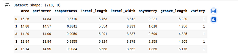Seeds dataset overview. (Image by Author)

Step 2: Data pre-processing

Let’s explore the data structure and prepare it for LDA analysis:

# Check for missing values
print(f"Missing values: {seeds_df.isnull().sum().sum()}")

# Check class distribution
print("\nClass distribution:")
print(seeds_df['variety'].value_counts())

# Separate features and target
X = seeds_df.drop('variety', axis=1)
y = seeds_df['variety']

# Split the data into training and testing sets
X_train, X_test, y_train, y_test = train_test_split(X, y, test_size=0.3,
                                                   random_state=42, stratify=y)

# Standardize the features
scaler = StandardScaler()
X_train_scaled = scaler.fit_transform(X_train)
X_test_scaled = scaler.transform(X_test)

Here, we’re checking if the dataset has any missing values and examining how many examples belong to each category. Then, we prepare the data by separating inputs from labels, splitting it into training and test portions, and standardizing the input values so that all features are on a similar scale.

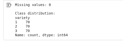
Data pre-processing. (Image by Author)

We see that there are no missing values, and the class distribution is equal.

Step 3: Applying LDA for dimensionality reduction

Now we’ll apply LDA to reduce the dimensionality of our data while preserving class separability:

# Create and fit LDA model
lda = LinearDiscriminantAnalysis(n_components=2)
X_train_lda = lda.fit_transform(X_train_scaled, y_train)
X_test_lda = lda.transform(X_test_scaled)

# Print explained variance ratio
print("Explained variance ratio:", lda.explained_variance_ratio_)
print("Cumulative explained variance:", np.cumsum(lda.explained_variance_ratio_))

We’re creating a model that finds the best directions to separate the different categories in our data. By reducing the data to two new features (since we have three categories), we keep the most important patterns for distinguishing between them.

The output is as follows:

LDA variance results. (Image by Author)

This output shows how much of the class-separating information is captured by the two new features created by LDA:

• Explained variance ratio: This means the first LDA component captures about 67.7% of the information needed to distinguish between the classes, while the second component captures the remaining 32.3%.
• Cumulative explained variance: Together, both components capture 100% of the class-separating information in the original data. This is expected since we have 3 classes, and LDA gives at most 2 useful directions.

Step 4: Visualize the LDA transformation

Let’s visualize how LDA transforms our data and separates the classes:

fig, (ax1, ax2) = plt.subplots(1, 2, figsize=(14, 6))

# Plot the first two original features
ax1.scatter(X_train_scaled[:, 0], X_train_scaled[:, 1],
           c=y_train, cmap='viridis', alpha=0.7, edgecolor='k')
ax1.set_xlabel('Area (standardized)')
ax1.set_ylabel('Perimeter (standardized)')
ax1.set_title('Original Feature Space (First Two Features)')
ax1.grid(True, alpha=0.3)

# Plot LDA-transformed data
scatter = ax2.scatter(X_train_lda[:, 0], X_train_lda[:, 1],
                     c=y_train, cmap='viridis', alpha=0.7, edgecolor='k')
ax2.set_xlabel('First Linear Discriminant')
ax2.set_ylabel('Second Linear Discriminant')
ax2.set_title('LDA-Transformed Space')
ax2.grid(True, alpha=0.3)

plt.colorbar(scatter, ax=ax2, label='Wheat Variety')
plt.tight_layout()
plt.show()

The code above creates two side-by-side charts to help us compare what the data looks like before and after applying the dimensionality reduction technique, as seen below:

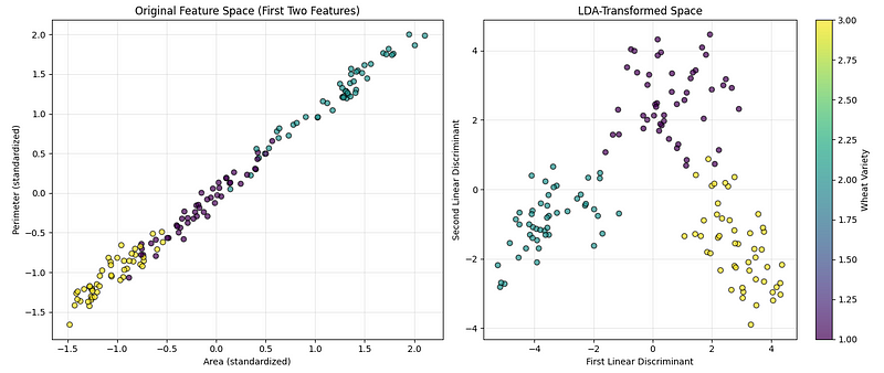LDA visualization. (Image by Author)

The first chart shows the original data using two of the measured features (area and perimeter), so we can see how well the categories are separated naturally. The second chart shows the data after transforming it into the most informative directions for separating the categories. A colorbar is added to show which color represents which type of wheat.

Step 5: Use LDA for classification

LDA can also be used directly as a classifier. 

Let’s implement it:

# Create LDA classifier
lda_classifier = LinearDiscriminantAnalysis()
lda_classifier.fit(X_train_scaled, y_train)

# Make predictions
y_pred = lda_classifier.predict(X_test_scaled)

# Calculate accuracy
accuracy = accuracy_score(y_test, y_pred)
print(f"Classification Accuracy: {accuracy:.4f}")

# Print classification report
print("\nClassification Report:")
print(classification_report(y_test, y_pred))

We’re training a model to recognize the different categories of wheat based on the training data. Then we test how well it performs on new, unseen examples by checking its overall accuracy and how well it predicts each category.

We see the following output:

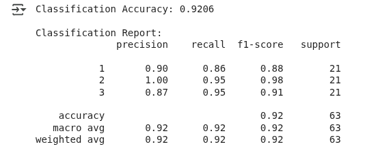
LDA classification results. (Image by Author)

The model correctly predicted the wheat type about 92% of the time, which can be considered a good performance. 

This example has demonstrated that while LDA is commonly used for dimensionality reduction, it can also act as a classifier by modeling the probability distribution of each class and assigning new data to the class with the highest likelihood.

Comparing LDA vs. PCA with Codes and Visualizations

Principal Component Analysis is another popular dimensionality reduction technique that finds the directions of maximum variance in the data. 

Let’s extend our earlier example to compare LDA with PCA:

from sklearn.decomposition import PCA

# Apply PCA with 2 components
pca = PCA(n_components=2)
X_train_pca = pca.fit_transform(X_train_scaled)
X_test_pca = pca.transform(X_test_scaled)

# Create comparison visualization
fig, (ax1, ax2) = plt.subplots(1, 2, figsize=(14, 6))

# Plot PCA results
scatter1 = ax1.scatter(X_train_pca[:, 0], X_train_pca[:, 1],
                      c=y_train, cmap='viridis', alpha=0.7, edgecolor='k')
ax1.set_xlabel('First Principal Component')
ax1.set_ylabel('Second Principal Component')
ax1.set_title(f'PCA Transformation\nExplained Variance: {pca.explained_variance_ratio_.sum():.2%}')
ax1.grid(True, alpha=0.3)

# Plot LDA results
scatter2 = ax2.scatter(X_train_lda[:, 0], X_train_lda[:, 1],
                      c=y_train, cmap='viridis', alpha=0.7, edgecolor='k')
ax2.set_xlabel('First Linear Discriminant')
ax2.set_ylabel('Second Linear Discriminant')
ax2.set_title(f'LDA Transformation\nExplained Variance: {lda.explained_variance_ratio_.sum():.2%}')
ax2.grid(True, alpha=0.3)

plt.colorbar(scatter1, ax=ax1, label='Wheat Variety')
plt.colorbar(scatter2, ax=ax2, label='Wheat Variety')
plt.tight_layout()
plt.show()

We see the following plot:

LDA vs. PCA comparision. (Image by Author)

The left chart shows the data using PCA, which finds the directions that capture the most overall variation in the data. The right chart shows the result of LDA, which finds the directions that best separate the wheat categories.

Based on our implementation results and the explained variance values, we can conclude that while both perform well, for classification problems like this, LDA usually creates a clearer separation between groups.

What distinguishes LDA from other dimensionality reduction techniques is its supervised nature. While PCA only considers the variance in the data without regard to class labels, LDA explicitly uses class information to find the most discriminative directions. This is ideal when dealing with high-dimensional data where class separability is more important than preserving overall variance.

Thus, PCA can be used when:

• We need unsupervised dimensionality reduction
• Class labels are unavailable or irrelevant
• We want to visualize high-dimensional data
• We need to reduce noise and computational complexity

Similarly, we can use LDA when:

• We have labeled data and want to maximize class separation
• The number of samples per class is sufficient (generally > 30)
• We need both dimensionality reduction and classification
• Class discrimination is more important than preserving overall variance

Pros and Cons of LDA

Like any algorithm, LDA has its strengths and limitations that we have to be mindful of before applying it in our projects.

Advantages

• Supervised learning advantage: Unlike PCA, LDA uses class label information to find the most discriminative features, making it more effective for classification tasks.
• Dimensionality reduction with classification: Serves a dual purpose of reducing dimensions while providing a built-in classifier.
• Computational efficiency: Requires only eigenvalue decomposition, making it fast even for moderately large datasets.
• Interpretability: The linear discriminants can be interpreted as weighted combinations of original features.
• Optimal for Gaussian distributions: It provides the optimal linear classifier when classes follow Gaussian distributions with equal covariance matrices.
• No hyperparameter tuning: Unlike many machine learning algorithms, LDA has no hyperparameters to tune for basic implementation.

Disadvantages

• Linear boundaries only: Cannot capture non-linear relationships between features and classes.
• Gaussian and equal covariance assumption: Assumes that each class follows a multivariate Gaussian distribution, which may not hold for real data, and assumes all classes have the same covariance matrix, which is often violated in practice.
• Limited components: Can extract at most (n_classes — 1) discriminant components, which may be insufficient for visualization in multi-class problems.
• Sensitive to outliers and multicollinearity issues: The mean and covariance calculations are sensitive to outliers, and the algorithm can perform poorly when features are highly correlated.
• Sample size requirements: Requires sufficient samples per class to estimate covariance matrices reliably.

Understanding these trade-offs helps us determine if LDA is the best algorithm to apply to the problem at hand.

Conclusion

This article introduced linear discriminant analysis, a supervised technique that combines dimensionality reduction with classification by maximizing the ratio of between-class to within-class scatter.

We explored the mathematical foundations of LDA, implemented it using Python, and compared it with PCA to understand when each technique is most appropriate. We also learned about LDA’s real-world applications and discussed its advantages and limitations.

To deepen your understanding of LDA and related machine learning techniques, consider enrolling in our Supervised Machine Learning in Python track, where you’ll master various algorithms and their implementations, or our Dimensionality Reduction in Python course to dive deeper into both supervised and unsupervised dimension reduction techniques.