Linear Regression in Python: Your Guide to Predictive Modeling

Python, with its rich ecosystem of libraries like NumPy, statsmodels, and scikit-learn, has become the go-to language for data scientists. Its ease of use and versatility make it perfect for both understanding the theoretical underpinnings of linear regression and implementing it in real-world scenarios.

In this guide, I'll walk you through everything you need to know about linear regression in Python. We'll start by defining what linear regression is and why it's so important. Then, we'll look into the mechanics, exploring the underlying equations and assumptions. You'll learn how to perform linear regression using various Python libraries, from manual calculations with NumPy to streamlined implementations with scikit-learn. We'll cover both simple and multiple linear regression, and I'll show you how to evaluate your models and enhance their performance.

What is Linear Regression?

Linear regression is a statistical method used to model the relationship between a dependent variable (target) and one or more independent variables (predictors). The objective is to find a linear equation that best describes this relationship.

Linear regression is widely used for predictive modeling, inferential statistics, and understanding relationships in data. Its applications include forecasting sales, assessing risk, and analyzing the impact of different variables on a target outcome.

What is simple linear regression?

For simple linear regression, this would take the form of a line in two-dimensional space; for multiple linear regression (with two independent variables), the relationship is represented by a plane in three-dimensional space; For even more independent variables, the equation describes a hyperplane in higher-dimensional space.

Let’s start with a simple linear regression model, which, as I mentioned, has only one predictor variable. It is represented by this equation:

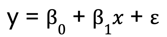
Where:

• y is the dependent variable,
• x is the independent variable,
• B₀ is the intercept,
• B₁ is the coefficient (slope) of the independent variable,
• represents the error term.

What is multiple linear regression?

In contrast, multiple linear regression extends this concept to include multiple predictor variables:

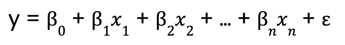
Where:

• 0 is the intercept,
• x₁, x₂, ..., x_n are the predictor variables
• 1,2, ..., n are the coefficients corresponding to each predictor variable,
• is the error term.

The Mechanics Behind Linear Regression

To understand how linear regression works, let’s break down its key components.

The linear model equation

We saw equations for linear regression, above, both with a single and multiple predictors. But now, let me talk about an important aspect of the equations. 

The term linear in linear regression refers to the functional form of the model, not necessarily the shape of the data. Specifically, it means that:

1. The model is linear in its parameters. This means each predictor is multiplied by a coefficient and summed.
2. The relationship between the dependent variable and predictors is additive, meaning changes in each predictor have a consistent effect on the dependent variable.
3. No exponentiation, multiplication between variables, or nonlinear transformations are applied to the parameters.

Ordinary least squares (OLS) method

To determine the best-fitting line, linear regression uses the ordinary least squares (OLS) method. OLS minimizes the sum of squared errors:

OLS minimizes the sum of squared errors:

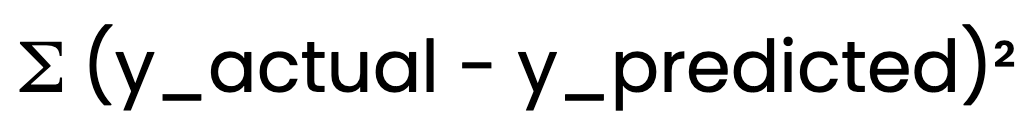
This ensures that the model provides the best possible estimates of B₀ and B₁.

Assumptions of linear regression

For linear regression to produce reliable results, certain assumptions must be met:

1. Linearity: The relationship between the independent and dependent variable should be linear.
2. Independence of Errors: The residuals (errors) should not be correlated with each other.
3. Constant Variance (Homoscedasticity): The spread of residuals should remain constant across all values.
4. Normality of Residuals: The residuals should follow a normal distribution.

Validating these assumptions ensures that our model is both reliable and valid. For example, if the relationship between variables is not linear, the model’s predictions may be inaccurate. If there is heteroscedasticity, the confidence intervals could be wrong.

Ways to Do Linear Regression in Python

Linear regression can be implemented in Python using different approaches. I'll walk you through three common methods: manual calculations with NumPy, detailed statistical modeling with statsmodels, and streamlined machine learning with scikit-learn.

Manual calculation approach (NumPy)

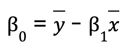
For a simple linear regression (one predictor variable), you can manually calculate the regression parameters using NumPy. This involves first calculating the mean of the independent and dependent variables. We then compute the slope (B₀):

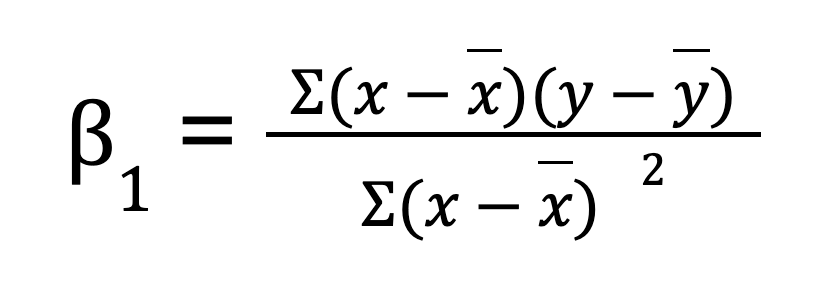
Once we have the slope, we can determine the intercept (B₁):

import numpy as np

# Sample data
x = np.array([1, 2, 3, 4, 5])
y = np.array([2, 4, 5, 4, 5])

# Compute means
x_mean = np.mean(x)
y_mean = np.mean(y)

# Compute slope (B1)
B1 = np.sum((x - x_mean) * (y - y_mean)) / np.sum((x - x_mean) ** 2)

# Compute intercept (B0)
B0 = y_mean - B1 * x_mean

print(f"Slope (B1): {B1}")
print(f"Intercept (B0): {B0}")

# Predicting values
y_pred = B0 + B1 * x
print("Predicted values:", y_pred)

If you're interested in simplifying the process, NumPy also provides a built-in function np.polyfit(), which can perform linear regression for you with just one line of code.

# Example of NumPy's polyfit
np.polyfit(x, y, 1)  # 1 stands for the degree of the polynomial (linear)

While this method is useful for understanding the math behind simple linear regression, it is impractical for large datasets, has less numerical precision, and doesn’t work for multiple regression problems.

Using a statistical library (statsmodels)

A more efficient way to perform linear regression is by using statsmodels, a library that provides statistical models and analysis tools.

Steps to fit an Ordinary Least Squares (OLS) model using Statsmodels:

1. Prepare the data: Ensure the independent variable is structured properly.

2. Add a constant: This accounts for the intercept term in the equation.

3. Fit the model: Use OLS() from statsmodels to estimate regression parameters.

4. Analyze the results: The .summary() function provides detailed model insights, including coefficients, p-values, and R-squared values.

import numpy as np
import statsmodels.api as sm

# Sample data
x = np.array([1, 2, 3, 4, 5])
y = np.array([2, 4, 5, 4, 5])

# Add constant for intercept term
X = sm.add_constant(x)

# Fit OLS model
model = sm.OLS(y, X).fit()

# Print summary
print(model.summary())

Using a machine learning library (scikit-learn)

scikit-learn is widely used because of its simplicity, scalability, and integration with other machine learning tools. It offers a simple and efficient way to perform linear regression using the LinearRegression class.

1. Import the library and load your dataset.

2. Reshape the predictor variable if necessary (for single-variable regression).

3. Create a model instance using LinearRegression().

4. Fit the model to the training data.

5. Retrieve the model parameters: The .coeff_ attribute returns the slope, while .intercept_ provides the intercept.

import numpy as np
from sklearn.linear_model import LinearRegression

# Sample data
x = np.array([1, 2, 3, 4, 5]).reshape(-1, 1)  # Reshape for scikit-learn
y = np.array([2, 4, 5, 4, 5])

# Create model instance
model = LinearRegression()

# Fit the model
model.fit(x, y)

# Get model parameters
print(f"Slope (B1): {model.coef_[0]}")
print(f"Intercept (B0): {model.intercept_}")

# Predict values
y_pred = model.predict(x)
print("Predicted values:", y_pred)

Other important methods

Beyond NumPy, statsmodels, and scikit-learn, several other Python libraries provide regression capabilities:

• Pandas: Useful for exploratory data analysis and quick trend modeling.
• SciPy: Includes statistical functions that can be used for regression analysis.
• TensorFlow & PyTorch: While primarily for deep learning, they can handle linear regression tasks effectively.

Each approach has its advantages. It depends on the complexity of your regression task.

Linear Regression in Python with One or More Predictors

Linear regression can handle both simple and complex relationships. In this section, we'll explore how to implement linear regression with one predictor (simple) and multiple predictors (multiple) using Python.

Simple linear regression in Python

For a simple linear regression in Python, we follow these steps:

Step 1: Compute the correlation

The correlation coefficient measures the strength of the relationship between x and y. We find it using NumPy:

import numpy as np

# Sample data
x = np.array([1, 2, 3, 4, 5])  # Independent variable
y = np.array([2, 4, 5, 4, 5])  # Dependent variable

correlation = np.corrcoef(x, y)[0, 1]
print("Correlation:", correlation)

Step 2: Compute the slope and intercept

The slope B₁ is computed as:

beta_1 = correlation * (np.std(y) / np.std(x))

You might notice that this equation looks slightly different from the earlier one, where I found the slope by summing the products of deviations between $x$ and y, then dividing by the sum of squared deviations in $x$. This new method, using correlation and standard deviation, may seem different but is actually the same. By rewriting the earlier equation, we can express the slope as $r$ multiplied by the ratio of the standard deviations of $y$ and $x$, making the two forms algebraically equivalent.

Now, for the intercept:

beta_0 = np.mean(y) - beta_1 * np.mean(x)

Step 3: Make predictions using the computed parameters

Now that we have the coefficients, we can find the predicted values.

y_pred = beta_0 + beta_1 * x

Going through these steps, I think, is helpful to understand the underlying calculations before using libraries like scikit-learn.

Multiple linear regression in Python

Multiple linear regression extends the concept of simple linear regression to model relationships between a dependent variable and multiple independent variables. This allows us to analyze more complex datasets where one predictor alone does not sufficiently explain the variation in the dependent variable.

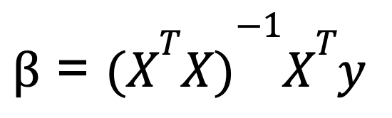
To perform multiple linear regression in Python, we typically use matrix algebra to calculate the coefficients that minimize the residual sum of squares. One commonly taught formula for calculating the coefficients in multiple linear regression is known as the normal equation:

Where:

• X is the matrix of independent variables (with a column of ones for the intercept),
• y is the vector of dependent variable values.
• X^T is the transpose of the matrix of X.
• (X^TX)^-1 is the inverse of X^TX.

This equation gives the optimal values for the coefficients that minimize the sum of squared errors.

Here’s an example of performing multiple linear regression with Python, using NumPy for the matrix operations:

import numpy as np

# Sample data: two predictors and one dependent variable
X = np.array([[1, 1], [1, 2], [2, 2], [2, 3]])  # Independent variables
y = np.array([6, 8, 9, 11])  # Dependent variable

# Add a column of ones to include the intercept in the model
X = np.column_stack((np.ones(X.shape[0]), X))

# Calculate beta coefficients using the normal equation
beta = np.linalg.inv(X.T @ X) @ X.T @ y
print("Coefficients:", beta)

This method works well when the predictors are independent, but if predictors are highly correlated, matrix inversion becomes unstable. For this reason, libraries like scikit-learn use a more numerically stable method based on QR decomposition to compute regression coefficients. So, even though we can calculate the coefficients using the normal equation, know that when we use the LinearRegression() function from scikitlearn, qr decomposition is working under the hood.

Addressing multicollinearity

Now is a good time to mention one thing that shows up as a concern in multiple linear regression in Python. Multicollinearity happens when two or more independent variables are highly correlated, making it difficult to isolate their individual effects. This can lead to unstable coefficient estimates. To detect and mitigate multicollinearity, you can calculate the variance inflation factor (VIF). You can also remove highly correlated variables, or else you can use regularization techniques like ridge regression and lasso regression.

Linear Regression Model Diagnostics and Evaluation in Python

After building your linear regression model, the next step is to evaluate its performance and validate that it meets the underlying assumptions. This ensures the reliability of your predictions and helps you identify potential improvements.

Residual analysis

Residual analysis is a core part of linear regression diagnostics. It helps to check the assumptions of linear regression and identify any violations. The residuals should be randomly scattered around zero, with no discernible pattern. Here's where visual tools like residual plots and Q-Q plots come into play:

1. Residual Plot: A scatter plot of the residuals versus the predicted values (or independent variables) helps to check if there’s any relationship that the model hasn’t accounted for. Ideally, the plot should show a random spread with no clear pattern, which suggests that the model has captured the linear relationship well.
2. Q-Q Plot (Quantile-Quantile Plot): A Q-Q plot helps to assess whether the residuals follow a normal distribution. For linear regression to be valid, the residuals should be approximately normally distributed. A straight line on the Q-Q plot indicates normality.

In Python, we can create these plots easily with libraries like matplotlib, seaborn, and statsmodels.

import numpy as np
import matplotlib.pyplot as plt
import seaborn as sns
import statsmodels.api as sm

# Sample data and linear regression model
X = np.array([[1, 1], [1, 2], [2, 2], [2, 3]])  # Independent variables
y = np.array([6, 8, 9, 11])  # Dependent variable

# Add an intercept term
X = sm.add_constant(X)

# Fit the linear regression model
model = sm.OLS(y, X).fit()

# Get the residuals
residuals = model.resid

# 1. Residual Plot
plt.figure(figsize=(10, 5))
plt.subplot(1, 2, 1)
plt.scatter(model.fittedvalues, residuals)
plt.axhline(y=0, color='r', linestyle='--')
plt.xlabel('Fitted Values')
plt.ylabel('Residuals')
plt.title('Residual Plot')

# 2. Q-Q Plot
plt.subplot(1, 2, 2)
sm.qqplot(residuals, line ='45', ax=plt.gca())
plt.title('Q-Q Plot')

plt.tight_layout()
plt.show()

Evaluation metrics

Apart from visual analysis, quantitative metrics are essential for assessing how well the linear regression model fits the data. Some key evaluation metrics include:

1. R-squared (R²): This metric tells you how much of the variance in the dependent variable can be explained by the independent variables. An R² value closer to 1 indicates that the model explains a large proportion of the variance, while a value closer to 0 means the model doesn’t fit the data well.
2. Adjusted R-squared: This metric adjusts R² for the number of predictors in the model. It is useful for comparing models with different numbers of predictors.
3. Root Mean Squared Error (RMSE): RMSE measures the average magnitude of the errors in the model’s predictions, with the same units as the dependent variable. A lower RMSE indicates better predictive performance.
4. Mean Absolute Error (MAE): MAE measures the average magnitude of the errors in the model’s predictions, but unlike RMSE, it does not penalize large errors as heavily. It's easier to interpret since it’s in the same units as the dependent variable.

These metrics can be easily computed in Python using statsmodels or scikit-learn:

from sklearn.metrics import mean_squared_error, mean_absolute_error, r2_score
import numpy as np

# Make predictions using the model
y_pred = model.predict(X)

# R-squared
r_squared = r2_score(y, y_pred)
print("R-squared:", r_squared)

# Adjusted R-squared (calculated manually)
n = len(y)  # number of data points
p = X.shape[1] - 1  # number of predictors (excluding intercept)
adj_r_squared = 1 - (1 - r_squared) * (n - 1) / (n - p - 1)
print("Adjusted R-squared:", adj_r_squared)

# RMSE
rmse = np.sqrt(mean_squared_error(y, y_pred))
print("Root Mean Squared Error (RMSE):", rmse)

# MAE
mae = mean_absolute_error(y, y_pred)
print("Mean Absolute Error (MAE):", mae)

By evaluating these metrics, you gain insights into the model’s accuracy, the goodness of fit, and how well the model generalizes to new data.

Enhancing Your Regression Model

Once you've evaluated your linear regression model, the next step is to explore ways to improve its performance. One common approach is through feature transformations, which can address non-linear relationships and help the model better capture underlying patterns in the data.

Feature transformations

Remember that, in linear regression, the model assumes a linear relationship between the independent variables (predictors) and the dependent variable. However, many real-world data sets have non-linear relationships that a simple linear model may not capture well. By applying feature transformations, such as logarithmic or square root transformations, you can sometimes improve the model's performance.

Logarithmic transformation

This is often used when a feature exhibits exponential growth or has large positive values. For example, transforming highly skewed income data (where a few very high-income values dominate) can make the distribution more normal.

import numpy as np
df['log_income'] = np.log(df['income'] + 1)  # +1 to avoid log(0)

Square root transformation

This is useful for features that follow a quadratic relationship. For example, a feature that represents counts (such as the number of visits to a website) may benefit from a square root transformation.

df['sqrt_visits'] = np.sqrt(df['visits'])

By transforming these features, you're helping the model better capture relationships that were previously missed by the linear approach. The key is to test different transformations and observe the effect on model performance. It's not a one-size-fits-all approach, and it requires empirical testing.

Normalization and standardization

In addition to feature transformations, it’s also important to understand the impact of normalization and standardization on your regression model, especially when you're dealing with features that have different units or scales. Normalization rescales the feature values to a range, typically [0, 1]. Standardization rescales the features to have a mean of 0 and a standard deviation of 1.

When you have multiple predictors, normalizing or standardizing the data helps to interpret the coefficients in a more meaningful way. That is, t helps show how much each predictor variable contributes to the dependent variable relative to other predictors. This is especially useful when the predictors are on different scales.

Conclusion

Developing a strong understanding of linear regression requires continuous practice and exploration. To deepen your knowledge, consider learning more about handling multicollinearity, heteroscedasticity, and regularization techniques like Ridge and Lasso regression. Strengthening your grasp of QR decomposition and variance inflation factor can also enhance model diagnostics. Additionally, understanding normalization vs. standardization can improve feature scaling decisions.