Course

Introduction
Trustpilot has become a popular website for customers to review businesses and services. In this short tutorial, you'll learn how to scrape useful information off this website and generate some basic insights from it with the help of R. You will find that TrustPilot might not be as trustworthy as advertised.

More specifically, this tutorial will cover the following:
- You'll first learn how you can scrape Trustpilot to gather reviews;
- Then, you'll see some basic techniques to extract information off of one page: you'll extract the review text, rating, name of the author and time of submission of all the reviews on a subpage.
- With these tools at hand, you're ready to step up your game and compare the reviews of two companies (of your own choice): you'll see how you can make use of tidyverse packages such as
ggplot2anddplyr, in combination withxts, to inspect the data further and to formulate a hypothesis, which you can further investigate with theinferpackage, a package for statistical inference that follows the philosophy of the tidyverse.
On Trustpilot a review consists of a short description of the service, a 5-star rating, a user name and the time the post was made.

Your goal is to write a function in R that will extract this information for any company you choose.
Create a Scraping Function
First, you will need to load all the libraries for this task.
    # General-purpose data wrangling
    library(tidyverse)

    # Parsing of HTML/XML files
    library(rvest)

    # String manipulation
    library(stringr)

    # Verbose regular expressions
    library(rebus)

    # Eases DateTime manipulation
    library(lubridate)
Find all Pages
As an example, you can choose the e-commerce company Amazon. This is purely for demonstration purposes and is in no way related to the case study that you'll cover in the second half of the tutorial.
The landing page URL will be the identifier for a company, so you will store it as a variable.
url <-'http://www.trustpilot.com/review/www.amazon.com'
Most large companies have several review pages. On Amazon's landing page you can read off the number of pages, here it is 155.

Clicking on any one of the subpages reveals a pattern for how the individual URLs of a company can be addressed. Each of them is the main URL with ?page=n added, where n is the number of a review page, here any number between 1 and 155.
This is how your program should operate:
- Find the maximum number of pages to be queried
- Generate all the subpages that make up the reviews
- Scrape the information from each of them
- Combine the information into one comprehensive data frame
Let's start with finding the maximum number of pages. Generally, you can inspect the visual elements of a website using web development tools native to your browser. The idea behind this is that all the content of a website, even if dynamically created, is tagged in some way in the source code. These tags are typically sufficient to pinpoint the data you are trying to extract.
Since this is only an introduction, you can take the scenic route and directly look at the source code yourself.
HTML data has the following structure:
    < Tag  Attribute_1 = Value_1 Attribute_2 = Value_2 ...>
        The tagged data
        <\Tag>
To get to the data, you will need some functions of the rvest package. To convert a website into an XML object, you use the read_html() function. You need to supply a target URL and the function calls the webserver, collects the data, and parses it. To extract the relevant nodes from the XML object you use html_nodes(), whose argument is the class descriptor, prepended by a . to signify that it is a class. The output will be a list of all the nodes found in that way. To extract the tagged data, you need to apply html_text() to the nodes you want. For the cases where you need to extract the attributes instead, you apply html_attrs(). This will return a list of the attributes, which you can subset to get to the attribute you want to extract.
Let's apply this in practice. After a right-click on Amazon's landing page you can choose to inspect the source code. You can search for the number '155' to quickly find the relevant section.

You can see that all of the page button information is tagged as 'pagination-page' class. A function that takes the raw HTML of the landing page and extracts the second to last item of the pagination-page class looks like this:
    get_last_page <- function(html){

      pages_data <- html %>%
                      # The '.' indicates the class
                      html_nodes('.pagination-page') %>%
                      # Extract the raw text as a list
                      html_text()

      # The second to last of the buttons is the one
      pages_data[(length(pages_data)-1)] %>%
        # Take the raw string
        unname() %>%
        # Convert to number
        as.numeric()
    }
The step specific for this function is the application of the html_nodes() function which extracts all nodes of the pagination class. The last part of the function simply takes the correct item of the list, the second to last, and converts it to a numeric value.
To test the function, you can load the starting page using the read_html() function and apply the function you just wrote:
    first_page <- read_html(url)
    (latest_page_number <- get_last_page(first_page))
[1] 155
Now that you have this number, you can generate a list of all relevant URLs
list_of_pages <- str_c(url, '?page=', 1:latest_page_number)
You can manually check that the entries to list_of_pages are indeed valid and can be called via a web browser.
Extract the Information of One Page
You want to extract the review text, rating, name of the author and time of submission of all the reviews on a subpage. You can repeat the steps from earlier for each of the fields you are looking for.
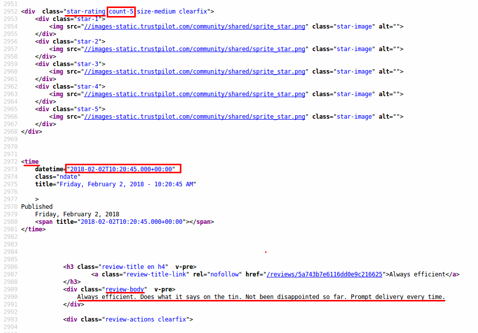
For each of the data fields you write one extraction function using the tags you observed. At this point a little trial-and-error is needed to get the exact data you want. Sometimes you will find that additional items are tagged, so you have to reduce the output manually.
    get_reviews <- function(html){
      html %>%
        # The relevant tag
        html_nodes('.review-body') %>%
        html_text() %>%
        # Trim additional white space
        str_trim() %>%
        # Convert the list into a vector
        unlist()
    }

    get_reviewer_names <- function(html){
      html %>%
        html_nodes('.user-review-name-link') %>%
        html_text() %>%
        str_trim() %>%
        unlist()
    }
The datetime information is a little trickier, as it is stored as an attribute.
In general, you look for the most broad description and then try to cut out all redundant information. Because time information not only appears in the reviews, you also have to extract the relevant status information and filter by the correct entry.
    get_review_dates <- function(html){

      status <- html %>%
                  html_nodes('time') %>%
                  # The status information is this time a tag attribute
                  html_attrs() %>%
                  # Extract the second element
                  map(2) %>%
                  unlist()

      dates <- html %>%
                  html_nodes('time') %>%
                  html_attrs() %>%
                  map(1) %>%
                  # Parse the string into a datetime object with lubridate
                  ymd_hms() %>%
                  unlist()

      # Combine the status and the date information to filter one via the other
      return_dates <- tibble(status = status, dates = dates) %>%
                        # Only these are actual reviews
                        filter(status == 'ndate') %>%
                        # Select and convert to vector
                        pull(dates) %>%
                        # Convert DateTimes to POSIX objects
                        as.POSIXct(origin = '1970-01-01 00:00:00')

      # The lengths still occasionally do not lign up. You then arbitrarily crop the dates to fit
      # This can cause data imperfections, however reviews on one page are generally close in time)

      length_reviews <- length(get_reviews(html))

      return_reviews <- if (length(return_dates)> length_reviews){
          return_dates[1:length_reviews]
        } else{
          return_dates
        }
      return_reviews
    }
The last function you need is the extractor of the ratings. You will use regular expressions for pattern matching. The rating is placed as an attribute of the tag. Rather than being just a number, it is part of a string count-X, where X is the number you want. Regular expressions can be a bit unwieldy, but the rebus package allows to write them in a nice human readable form. In addition, rebus' piping functionality, via the %R% operator, allows to decompose complex patterns into simpler subpatterns to structure more complicated regular expressions.
    get_star_rating <- function(html){

      # The pattern you look for: the first digit after `count-`
      pattern = 'count-'%R% capture(DIGIT)

      ratings <-  html %>%
        html_nodes('.star-rating') %>%
        html_attrs() %>%
        # Apply the pattern match to all attributes
        map(str_match, pattern = pattern) %>%
        # str_match[1] is the fully matched string, the second entry
        # is the part you extract with the capture in your pattern
        map(2) %>%

        unlist()

      # Leave out the first instance, as it is not part of a review
      ratings[2:length(ratings)]
    }
After you have tested that the individual extractor functions work on a single URL, you combine them to create a tibble, which is essentially a data frame, for the whole page. Because you are likely to apply this function to more than one company, you will add a field with the company name. This can be helpful in later analysis when you want to compare different companies.
    get_data_table <- function(html, company_name){

      # Extract the Basic information from the HTML
      reviews <- get_reviews(html)
      reviewer_names <- get_reviewer_names(html)
      dates <- get_review_dates(html)
      ratings <- get_star_rating(html)

      # Combine into a tibble
      combined_data <- tibble(reviewer = reviewer_names,
                              date = dates,
                              rating = ratings,
                              review = reviews)

      # Tag the individual data with the company name
      combined_data %>%
        mutate(company = company_name) %>%
        select(company, reviewer, date, rating, review)
    }
You wrap this function in a command that extracts the HTML from the URL such that handling becomes more convenient.
    get_data_from_url <- function(url, company_name){
      html <- read_html(url)
      get_data_table(html, company_name)
    }
In the last step, you apply this function to the list of URLs you generated earlier. To do this, you use the map() function from the purrr package which is part of the tidyverse. It applies the same function over the items of a list. You already used the function earlier, however, you passed a number n, which is short-hand for extracting the n-th sub-item of the list.
Finally, you write one convenient function that takes as input the URL of the landing page of a company and the label you want to give the company. It extracts all reviews, binding them into one tibble. This is also a good starting point for optimising the code. The map function applies the get_data_from_url() function in sequence, but it does not have to. One could apply parallelisation here, such that several CPUs can each get the reviews for a subset of the pages and they are only combined at the end.
    scrape_write_table <- function(url, company_name){

      # Read first page
      first_page <- read_html(url)

      # Extract the number of pages that have to be queried
      latest_page_number <- get_last_page(first_page)

      # Generate the target URLs
      list_of_pages <- str_c(url, '?page=', 1:latest_page_number)

      # Apply the extraction and bind the individual results back into one table,
      # which is then written as a tsv file into the working directory
      list_of_pages %>%
        # Apply to all URLs
        map(get_data_from_url, company_name) %>%
        # Combine the tibbles into one tibble
        bind_rows() %>%
        # Write a tab-separated file
        write_tsv(str_c(company_name,'.tsv'))
    }
You save the result to disk using a tab-separated file, instead of the common comma-separated files (CSVs), as the reviews often contain commas, which may confuse the parser.
As an example you can apply the function to Amazon:
    scrape_write_table(url, 'amazon')

    amz_tbl <- read_tsv('amazon.tsv')
    tail(amz_tbl, 5)
    # A tibble: 5 x 5
      company            reviewer                date rating
        <chr>               <chr>              <dttm>  <int>
    1  amazon            Anders T 2009-03-22 13:14:12      5
    2  amazon             David E 2008-12-31 18:57:31      5
    3  amazon      Joseph Harding 2008-09-16 13:05:05      3
    4  amazon   "Mads D\u00f8rup" 2008-04-28 11:09:05      5
    5  amazon Kim Fuglsang Kramer 2007-08-27 17:25:01      4
    # ... with 1 more variables: review <chr>
Case Study: A Tale of Two Companies
With the webscraping function from the previous section, you can quickly obtain a lot of data. With this data, many different analyses are possible.
In this case study, you'll only use meta-data of the reviews, namely their rating and the time of the review.
First, you load additional libraries.
    # For working with time series
    library(xts)

    # For hypothesis testing
    library(infer)
The companies you are interested in are both prominent players in the same industry. They both also use their TrustPilot scores as selling points on their website.
You have scraped their data and only need to load it:
    data_company_a <- read_tsv('company_A.tsv')
    data_company_b <- read_tsv('company_B.tsv')
You can summarise their overall numbers with the help of the group_by() and summarise() functions from the dplyr package:
    full_data <- rbind(data_company_a, data_company_b)

    full_data%>%
      group_by(company) %>%
      summarise(count = n(), mean_rating = mean(rating))
| company | count | mean_rating |
|---|---|---|
| company_A | 3628 | 4.908214 |
| company_B | 2615 | 4.852773 |
The average ratings for the two companies look comparable. Company B, which has been in business for a slightly longer period of time, also seems to have a slightly lower rating.
Comparing Time Series
A good starting point for further analysis is to look at how the month-by-month performance by rating was for each company. First, you extract time series from the data and then subset them to a point where both companies were in business and sufficient review activity is generated. This can be found by visualising the time series. If there are very large gaps in the data for several months on end, then conclusions drawn from the data is less reliable.
    company_a_ts <- xts(data_company_a$rating, data_company_a$date)
    colnames(company_a_ts) <- 'rating'
    company_b_ts <- xts(data_company_b$rating, data_company_b$date)
    colnames(company_b_ts) <- 'rating'

    open_ended_interval <- '2016-01-01/'

    # Subsetting the time series
    company_a_sts <- company_a_ts[open_ended_interval]
    company_b_sts <- company_b_ts[open_ended_interval]
You can now apply the monthly averaging with the apply.monthly() function from the xts package. To start, gather the mean monthly ratings for each company. Time series can have more than one observation for the same index. To specify that the average is taken with respect to one field, here rating, we have to pass colMeans.
Next, don't forget to pass in length to the FUN argument to retrieve the monthly counts. This is because the time series can be seen as a vector. Each review increases the length of that vector by one and the length function essentially counts the reviews.
    company_a_month_avg <-  apply.monthly(company_a_sts, colMeans, na.rm = T)
    company_a_month_count  <-  apply.monthly(company_a_sts, FUN = length)

    company_b_month_avg <-  apply.monthly(company_b_sts, colMeans, na.rm = T)
    company_b_month_count  <-  apply.monthly(company_b_sts, FUN = length)
Next, you can compare the monthly ratings and counts. It's very easily done by plotting the monthly average ratings for each company and the counts for those ratings for each company in separate plots and then arranging them in a grid:
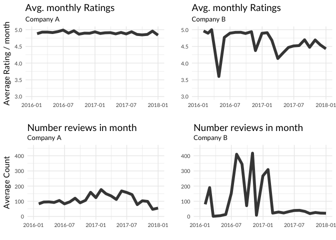
It seems company A has much more consistently high ratings. But not only that, for company B, the monthly number of reviews shows very pronounced spikes, especially after a bout of mediocre reviews.
Could there be chance of foul play?
Aggregate the Data Further
Now that you have seen that the data, especially for company B, changes quite dramatically over time, a natural question to ask how the review activity is distributed within a week or within a day.
    full_data <- full_data %>%
      filter(date >= start_date) %>%
      mutate(weekday = weekdays(date, abbreviate = T),
             hour = hour(date))

    # Treat the weekdays as factor.
    # The order is for the plotting only
    full_data$weekday <-  factor(full_data$weekday,
                                 levels = c('Mon', 'Tue', 'Wed', 'Thu', 'Fri', 'Sat', 'Sun'))
If you plot the reviews by week day and hour of the week, you also get remarkable differences:
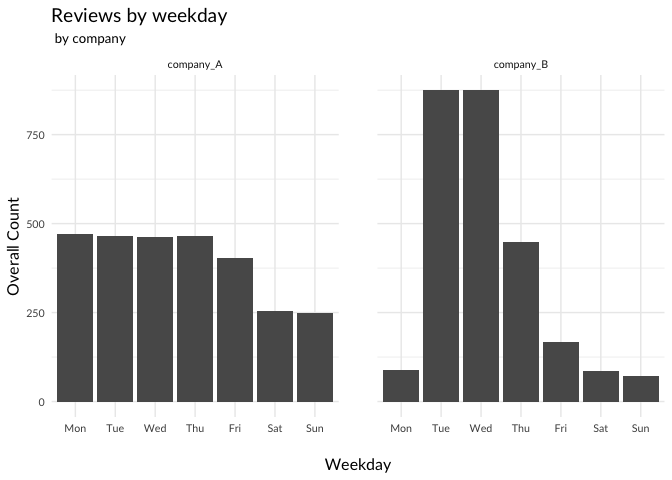
A splitting by time of the day of the reviews also shows striking differences between the two competitors:
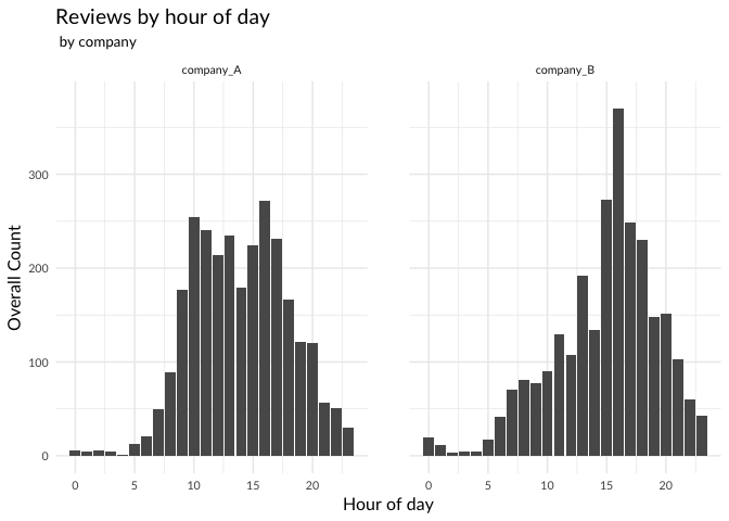
It looks as if more reviews are written during the day than at night. Company B however shows a pronounced peak in the reviews written in the afternoon.
The Null Hypothesis
These patterns seem to indicate that there is something fishy going on at company B. Maybe some of the reviews are not written by users, but rather by professionals. You would expect that these reviews are, on average, better than those that are written by ordinary people. Since the review activity for company B is so much higher during weekdays, it seems likely that professionals would write their reviews on one of those days. You can now formulate a null hypothesis which you can try to disprove using the evidence from the data.
There is no systematic difference between reviews written on a working day versus reviews written on a weekend.
To test this, you divide company B's reviews into those that are written on weekdays and those written on weekends, and check their average ratings
    hypothesis_data <- full_data %>%
      mutate(is_weekend = ifelse(weekday %in% c('Sat', 'Sun'), 1, 0)) %>%
      select(company, is_weekend, rating)

    hypothesis_data %>%
      group_by(company, is_weekend) %>%
      summarise(avg_rating = mean(rating)) %>%
      spread(key = is_weekend, value = avg_rating) %>%
      rename(weekday = '0', weekend = '1)
| company | weekday | weekend |
|---|---|---|
| company_A | 4.898103 | 4.912176 |
| company_B | 4.864545 | 4.666667 |
It certainly looks like a small enough difference, but is it pure chance?
You can extract the difference in averages:
    weekend_rating <- hypothesis_data %>%
      filter(company == 'company_B') %>%
      filter(is_weekend == 1) %>%
      summarise(mean(rating)) %>%
      pull()

    workday_rating <- hypothesis_data %>%
      filter(company == 'company_B') %>%
      filter(is_weekend == 0) %>%
      summarise(mean(rating)) %>%
      pull()

    (diff_work_we <- workday_rating - weekend_rating)
[1] 0.1978784
If there really was no difference between working days and weekends, then you could simply permute the is_weekend label and the difference between the averages should be of the same order of magnitude. A convenient way to do these sort of 'Hacker Statistics' is provided by the infer package:
    permutation_tests <- hypothesis_data %>%
      filter(company == 'company_B') %>%
      specify(rating ~ is_weekend ) %>%
      hypothesize(null = 'independence') %>%
      generate(reps = 10000, type = 'permute') %>%
      calculate(stat = 'diff in means', order = c(0,1))
Here you have specified the relation you want to test, your hypothesis of independence and you tell the function to generate 10000 permutations, calculating the difference in mean rating, for each. You can now calculate the frequency of the permutation producing, by chance, such a difference in mean ratings:
    permutation_tests %>%
      summarise(p = mean(abs(stat)>= diff_work_we))
    # A tibble: 1 x 1
          p
      <dbl>
    1 7e-04
Indeed, the chance of the observed effect being pure chance is exceedingly small. This does not prove any misdoing, however it is very suspicious. For example, doing the same experiment for company A gives a p value of 0.561, which means that its very likely to get a value as extreme as the one observed, which certainly does not invalidate your null hypothesis.
Conclusion: Don't Trust the Reviews (Blindly)
In this tutorial, you have written a simple program that allows you to scrape data from the website TrustPilot. The data is structured in a tidy data table and presents an opportunity for a large number of further analyses.
As an example, you scraped information for two companies that work in the same industry. You analysed their meta-data and found suspicious patterns for one. You used hypothesis testing to show that there is a systematic effect of the weekday on one company's ratings. This is an indicator that reviews have been manipulated, as there is no other good explanation of why there should be such a difference. You could not verify this effect for the other company, which however does not mean that their reviews are necessarily honest.
More information on review websites being plagued by fake reviews can be found for example in the Guardian.
Want to learn more about Web scraping in R? Check out our Web Scraping and Parsing Data in R tutorial.
