
Track
Developing AI Applications
21 hr
Microsoft’s RStar-math paper presents an innovative approach to solving mathematical problems using a combination of reinforcement learning, symbolic reasoning, and Monte Carlo Tree Search (MCTS).
In this blog, I'll explore the RStar framework and its core components. I'll then guide you step-by-step through a simplified implementation that demonstrates its key concepts using Gradio. While this demo is inspired by the paper, some complexities have been simplified for accessibility.
The RStar math aims to bridge symbolic reasoning with the generalization capabilities of pre-trained neural models. The framework integrates components like Monte Carlo Tree Search (MCTS), pre-trained language models, and reinforcement learning to enable efficient exploration of problem-solving strategies.
The core idea is to represent mathematical reasoning as a search process over a structured tree of possible steps, where each node represents a partial solution or state.
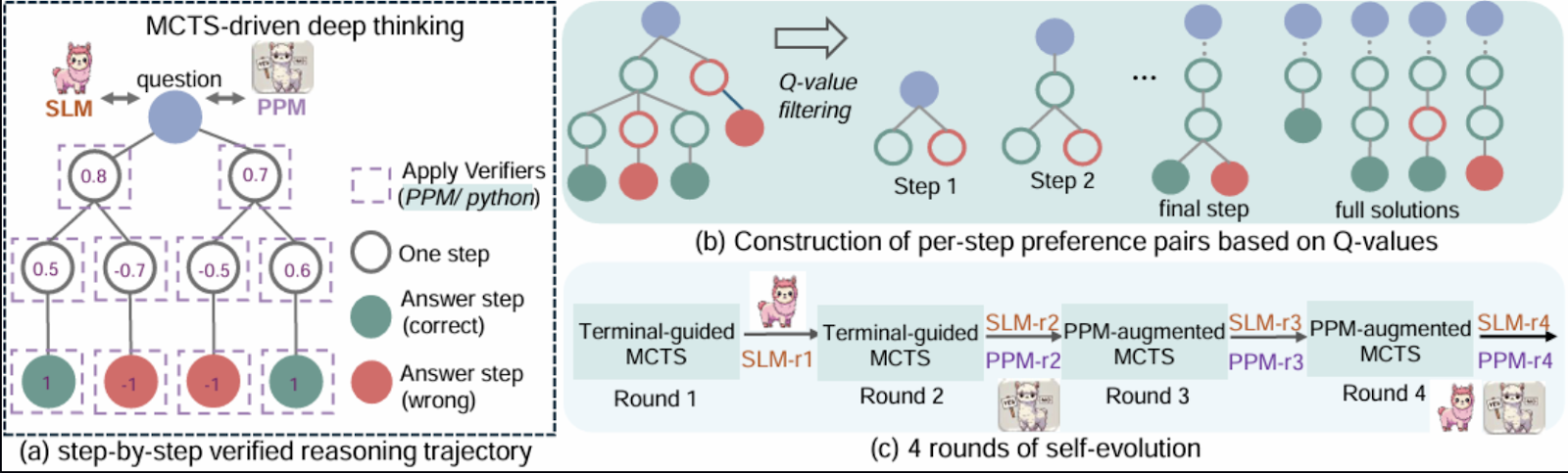
Source: Guan et al., 2025
Some of the reasons that make rStar-Math particularly interesting for me are:
The demo demonstrates how a policy model and a reward model, combined with symbolic reasoning using the sympy library, can tackle mathematical problems in a structured way. The key features of this implementation include:
To keep the demo simple and focused, certain advanced features pointed out in the paper are beyond the scope of this tutorial. Those features are:
The demo is broken into several components, each reflecting a part of the RStar methodology. Before we begin, ensure you have the following installed:
pip install requests gradio, sympy Then, import these libraries:
import gradio as gr
import numpy as np
import torch
import re
import torch.nn as nn
import torch.optim as optim
from sympy import symbols, Eq, solve, N, sin, cos, tan, exp, log, E, sympify
from random import choice
Now that all the dependencies are installed, let’s set up the main components.
These networks are lightweight versions of the models described in the paper, used to predict the next action and evaluate success. The policy model predicts the next steps to solve the given equations. It uses a feedforward neural network to process encoded representations of the problem.
Similarly, the reward model evaluates partial solutions to guide the MCTS process. Both models are implemented using PyTorch.
class PolicyModel(nn.Module):
    def __init__(self, input_size, hidden_size, output_size):
        super().__init__()
        self.fc1 = nn.Linear(input_size, hidden_size)
        self.fc2 = nn.Linear(hidden_size, output_size)
        self.relu = nn.ReLU()
    def forward(self, x):
        x = self.relu(self.fc1(x))
        x = self.fc2(x)
        return x
class RewardModel(nn.Module):
    def __init__(self, input_size, hidden_size, output_size):
        super().__init__()
        self.fc1 = nn.Linear(input_size, hidden_size)
        self.fc2 = nn.Linear(hidden_size, output_size)
        self.relu = nn.ReLU()
    def forward(self, x):
        x = self.relu(self.fc1(x))
        x = self.fc2(x)
        return x
Next, we build a node class for MCTS trees.
The TreeNode class represents nodes in the MCTS tree. Each node corresponds to a state in the search process, containing:
class TreeNode:
    """Represents a node in the MCTS tree."""
    def __init__(self, state, parent=None):
        self.state = state  # Current state
        self.parent = parent
        self.children = []
        self.visits = 0
        self.q_value = 0.0  # Accumulated rewards
    def is_fully_expanded(self):
        return len(self.children) > 0
    def best_child(self, exploration_weight=1.4):
        """Select the best child using UCT formula."""
        def uct_value(child):
            return (child.q_value / (child.visits + 1e-6)) + exploration_weight * np.sqrt(np.log(self.visits + 1) / (child.visits + 1e-6))
        return max(self.children, key=uct_value)
    def add_child(self, child_state):
        """Add a child node with the given state."""
        child = TreeNode(state=child_state, parent=self)
        self.children.append(child)
        return child
Now that we have the basic structure in place, we will work next with the core components of the demo.
The MathSolver class is the core of the demo, combining symbolic reasoning with neural-guided search. It implements several key components:
The PolicyModel predicts the next steps to solve equations, while the RewardModel evaluates the success of partial or complete solutions.
class MathSolver:
    def __init__(self, dataset=None):
        self.dataset = dataset or []  # Dataset of math problems
        self.policy_model = PolicyModel(input_size=128, hidden_size=64, output_size=4)
        self.reward_model = RewardModel(input_size=128, hidden_size=64, output_size=1)
        self.policy_optimizer = optim.Adam(self.policy_model.parameters(), lr=0.001)
        self.reward_optimizer = optim.Adam(self.reward_model.parameters(), lr=0.001)
        self.execution_context = {}
The above method initializes the MathSolver class by setting up the components required for solving mathematical problems. It optionally accepts a dataset of math problems and initializes two neural networks: the policy model, which predicts the next action, and the reward model, which evaluates the success of actions.
We now have a policy and reward function in place. Next, we need to parse and encode the input equations.
The equations are parsed using sympy and encoded into feature vectors for processing by the policy and reward models.
def encode_problem(self, problem):
 # Advanced encoding using symbolic representation and problem length
     variables = len(re.findall(r'[a-zA-Z]', problem))
     operators = len(re.findall(r'[\+\-\*/\^]', problem))
      problem_length = len(problem)
      return np.array([variables, operators, problem_length] + [0] * 125)
The encode_problem method converts a math problem into a fixed-size numerical representation for the models. It extracts features like the number of variables, operators, and problem length, encoding them into a 128-dimensional NumPy array. This representation captures the problem's structure, enabling effective model processing.
The following code generates the next steps for solving the given equations, including defining variables, creating equations, and solving them.
def policy_model_predict(self, equation1, equation2=None):
    try:
        equations = []
        if equation1:
            equations.append(sympify(equation1.strip()))  # Sympify only equations
        if equation2:
            equations.append(sympify(equation2.strip()))
        all_variables = set()
        for eq in equations:
            all_variables.update(eq.free_symbols)
        var_definitions = [f"{v} = symbols('{v}')" for v in all_variables]
        steps = [
            ("Define variables", "\n".join(var_definitions)),
            ("Define equation(s)", f"equations = {equations}"),
            ("Solve equation(s)", f"solution = solve(equations, {list(all_variables)})"),
            ("Print solution", "print(solution)")
        ]
        return steps
    except Exception as e:
        print(f"Error during policy model prediction: {e}")
        return []
The policy_model_predict function parses the input equations using SymPy's sympify to ensure they are valid mathematical expressions. It then identifies all the variables present in the equations and solves them using SymPy's solve function. This method serves as a high-level guide for the problem-solving workflow.
The reward_model_predict method plays a vital role in reinforcement learning by providing feedback for actions taken during Monte Carlo Tree Search (MCTS) rollouts.
  def reward_model_predict(self, steps, success):
        encoded_steps = self.encode_problem(str(steps))
        encoded_steps = torch.tensor(encoded_steps, dtype=torch.float32)
        reward = self.reward_model(encoded_steps)
        return reward.item() if success else -reward.item()
The function encodes problem-solving steps into a numerical format and evaluates them through the reward model, returning a positive reward for success and a negative reward for failure. This feedback trains the policy model, guiding it to prioritize effective actions and improve decision-making. With the policy and reward model prediction functions in place, we can now work on the execution task.
This method handles multi-variable solutions as tuples or dictionaries and converts symbolic results to numerical approximations using SymPy's N function.
    def execute_code(self, code):
        try:
            # Ensure necessary imports and variables are in the execution context
            exec("from sympy import symbols, Eq, solve, N, sin, cos, tan, exp, log, E", self.execution_context)
            # Dynamically initialize variables in the context
            for var_def in self.execution_context.get('var_definitions', []):
                exec(var_def, self.execution_context)
            exec(code, self.execution_context)
            if "solution" in self.execution_context:
                symbolic_solution = self.execution_context["solution"]
                # Handle multi-variable solutions as tuples
                if isinstance(symbolic_solution, list):
                    self.execution_context["solution"] = [tuple(map(N, sol)) if isinstance(sol, tuple) else N(sol) for sol in symbolic_solution]
                elif isinstance(symbolic_solution, dict):
                    self.execution_context["solution"] = {k: N(v) for k, v in symbolic_solution.items()}
                else:
                    self.execution_context["solution"] = N(symbolic_solution)
            return True
        except Exception as e:
            print(f"Error executing code: {e}")
            return False
This method ensures accurate computation and supports flexible handling of various solution formats. In case of errors, it logs the issue and returns False, maintaining robust error handling.
The MCTS method iteratively selects the best states, expands the search tree, and simulates possible solutions. Rewards from simulations are back-propagated to improve decision-making.
def mcts(self, equation1, equation2=None, num_rollouts=10):
    root = TreeNode(state=(equation1, equation2))
    for _ in range(num_rollouts):
        # Selection
        node = root
        while node.is_fully_expanded() and node.children:
            node = node.best_child()
        # Expansion
        if not node.is_fully_expanded():
            steps = self.policy_model_predict(*node.state)
            for step, code in steps:
                child_state = (step, code)
                node.add_child(child_state)
        # Simulation
        success = True
        for step, code in steps:
            if not self.execute_code(code):
                success = False
                break
        # Backpropagation
        reward = self.reward_model_predict(steps, success)
        while node:
            node.visits += 1
            node.q_value += reward
            node = node.parent
    return root.best_child().state if root.children else None
The mcts method iteratively performs four key steps:
policy_model_predict method.reward_model_predict method and propagated up the tree to update node values. After a specified number of rollouts, the method returns the state of the best child node, representing the most promising solution explored during the search.
The solve method orchestrates the entire process, from parsing equations to executing and validating solutions.
def solve(self, equation1, equation2=None):
    self.execution_context = {}
    steps = self.policy_model_predict(equation1, equation2)
    variables = set()
    for eq in [equation1, equation2] if equation2 else [equation1]:
        if eq:
            variables.update(sympify(eq.strip()).free_symbols)
    self.execution_context['var_definitions'] = [f"{v} = symbols('{v}')" for v in variables]
    steps_output = ["Best solution found:"]
    for step, code in steps:
        steps_output.append(f"Step: {step}")
        steps_output.append(f"Code: {code}")
        if self.execute_code(code):
            steps_output.append("Execution successful.")
        else:
            steps_output.append("Execution failed.")
    if "solution" in self.execution_context:
        final_answer = self.execution_context["solution"]
        if isinstance(final_answer, dict):
            for var, value in final_answer.items():
                steps_output.append(f"{var} = {value}")
        elif isinstance(final_answer, list):
            for solution in final_answer:
                if isinstance(solution, tuple):
                    for idx, var in enumerate(variables):
                        steps_output.append(f"{list(variables)[idx]} = {solution[idx]}")
                else:
                    steps_output.append(f"Solution: {solution}")
        else:
            steps_output.append(f"Final Answer: {final_answer}")
    else:
        steps_output.append("No final answer found.")
    return "\n".join(steps_output)
The solve method processes one or two user-provided equations by initializing an execution context and generating steps via policy_model_predict. It executes each step, logs progress, and reports success or failure. Solutions, including single and multivariable results, are formatted with variable names and values for clarity. If no solution is found, an appropriate message is displayed.
We have all the core components in place, so we can work on the Gradio app next.
The Gradio interface allows users to input equations (one or more), solve them, and view the results interactively.
with gr.Blocks() as app:
    gr.Markdown("# Math Problem Solver with Advanced Multi-Step Reasoning and Learning")
    with gr.Row():
        equation1_input = gr.Textbox(label="Enter the first equation (e.g., x + y - 3)", placeholder="x + y - 3")
        equation2_input = gr.Textbox(label="Enter the second equation (optional, e.g., x - y - 1)", placeholder="x - y - 1")
    solve_button = gr.Button("Solve")
    solution_output = gr.Textbox(label="Solution", interactive=False)
    solve_button.click(solve_math_problem, inputs=[equation1_input, equation2_input], outputs=[solution_output])
app.launch(debug=True)
The above code creates a Gradio user interface for solving mathematical equations with advanced reasoning. The interface is wrapped in a gr.Blocks container, which contains two input fields using gr.Textbox: one for the first equation (mandatory) and another for the second equation (optional).
The output is displayed in a single gr.Textbox labeled "Solution". The interface.launch() command launches the Gradio app in a browser, and the debug=True flag enables detailed logs to help troubleshoot errors.
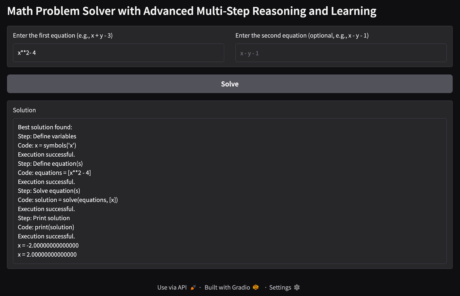
It’s time to test our Math Problem Solver app. Here are some tests I ran:
1. Single variable single equation: I tried to find possible values of a single variable x given a single equation as input.
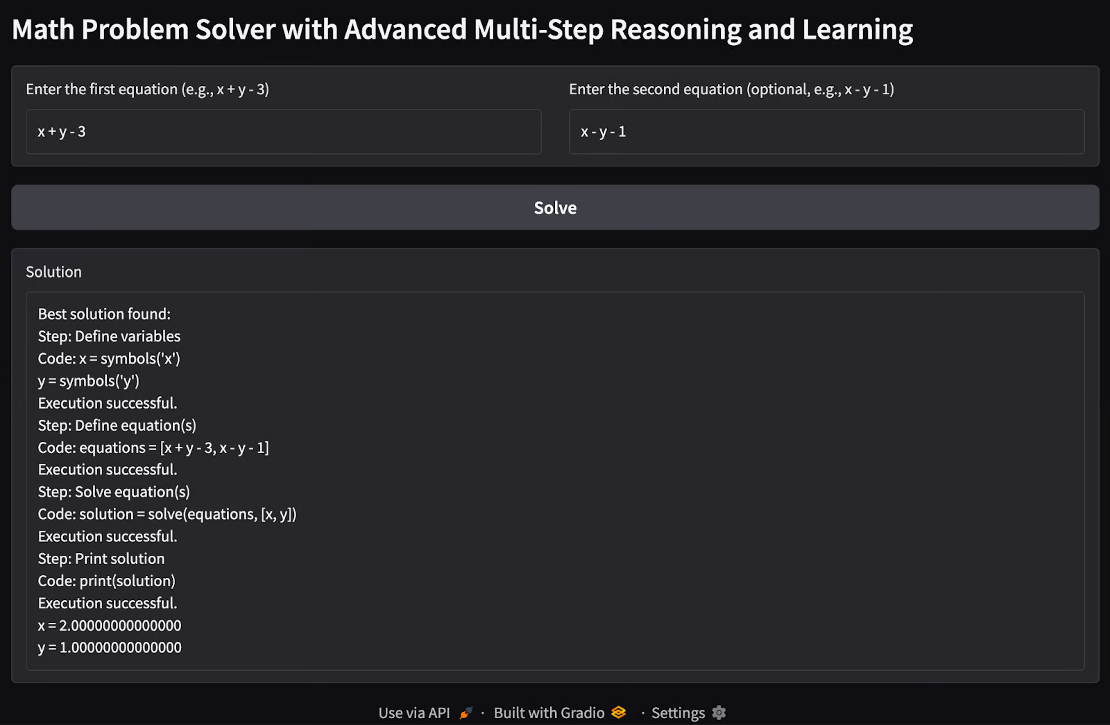
2. Multiple variable multiple equations problem: I passed in two equations with two variable problems to find possible values of variables x and y.
This demo is a basic version of what we can achieve with the capabilities of the rStar-math method. There is still a lot of work that can be done to extend its capabilities.
You can refer to the original repository of the rStar-math paper on GitHub.
This demo showcases a practical implementation of multi-step reasoning for solving mathematical equations. By combining neural networks, symbolic reasoning, and MCTS, it provides a glimpse into how advanced AI techniques can tackle structured reasoning tasks. Future enhancements could bring it closer to the full capabilities of the RStar framework.
Learn AI with these courses!
Track
Track
Track
Tutorial
Arunn Thevapalan
Tutorial
Hesam Sheikh Hassani
Tutorial
Aashi Dutt
Tutorial
Karlijn Willems
Tutorial
Karlijn Willems
Tutorial
Abid Ali Awan