Structural Equation Modeling: What It Is and When to Use It

Structural equation modeling (SEM) allows us to investigate causal relationships among variables and understand how each contributes to overall performance. SEM is a powerful tool that combines factor analysis and multiple regression analysis to analyze relationships among multiple variables. This is somewhat similar to how, in our daily lives, we consider how factors like posture, confidence, and communication skills collectively impact something like interview performance. 

Let’s now explore SEM, its applications, and practical examples in Python. If you are new to some of the central ideas, such as the idea of latent factors, you can also try our Factor Analysis course.

What is Structural Equation Modeling?

Structural equation modeling represents the causal relationships between latent and observed variables. The observed variables are what we can measure directly. Latent constructs are inferred and not measured directly. 

To effectively capture these relationships, SEM is divided into two main components:: the measurement model and the structural model. The measurement model specifies the relationships between observed variables and their corresponding latent variables, while the structural model specifies the relationships between latent variables.

Why do researchers use structural equation modeling? 

Statistical techniques like correlation and regression are inefficient in studying complex multivariate relationships. SEM is suitable for modeling complex, multifaceted constructs that are measured with error. It is also useful because it helps specify a system of relationships. Traditional methods help us study an independent variable and a set of predictors. While correlation is not causation, SEM helps us understand the causal relationship between the observed variable and latent constructs.

Some of the applications of SEM include:

• Social Science: SEM can be used to study the influence of cultural values on human behaviour in different societies.
• Education: SEM can be used to investigate students' experience in graduate schools. For example, to model the dropout rates for PhD students in the US. 
• Disease Risk Modeling: SEM can be applied to disease risk modelling to determine the risk of diseases like diabetes or heart disease.

Structural equation modeling core concepts

Here are some of the core concepts in structural equation modeling: 

• Observed Variables: Observed variables are directly measured from the study. Examples are responses to questionnaire fields.
• Latent Variables: Latent variables are inferred from the observed variables in the study. For example, the level of intelligence in a student's academic performance rating.
• Endogenous Variables: They are also known as dependent variables. For example, in y = x1 + x2 + x3, y is the endogenous variable as it depends on the values of x1, x2, …, xn.
• Exogenous Variables: They are independent variables. For example, an athlete’s sleep time is independent of the type of racing bike. 
• Measurement Model: measures the relationships between latent constructs and observed variables. The confirmatory factor analysis framework tests the underlying hypothesis of the measurement model.
• Structural Model: This model investigates causal relationships between latent constructs. It is diagrammatically represented using path analysis.

Structural equation modeling statistical assumptions

While SEM is great for modeling casual relationships, it has some underlying assumptions on the data. The assumptions include:

1. Linearity: SEM assumes linear relationships between the latent constructs and the observed variables. It is not suitable for non-linear datasets as it can give incorrect results. 
2. Multicollinearity: SEM assumes minimal multicollinearity between the observed variables. For example, a competitor’s sleep time and nutrition might be highly correlated. SEM assumes little correlation between these variables.
3. Sampling Assumptions: For SEM tasks, you need a sufficient sample size of at least 200 for good results. While you don’t need large datasets like LLMs, a smaller sample size can give inaccurate results.
4. Multivariate Normality: SEM assumes the data is a multivariate normal distribution. It is not suitable for non-normal data. You can perform tests to check for normality.
5. Missing Data: SEM assumes that the data is complete. One way SEM approaches missing data is to assume that the data is missing at random. Missing data might interfere with the model’s estimate.
6. Specification Error: SEM assumes that the defined model is specified correctly. It assumes that the measurement and structural models are assumed to contain at least all the relevant variables.

Types of structural equation models

There are different types of structural equation modeling. In no particular order, they are:

• Path Analysis: It is a type of SEM and an extension of regression models that deals only with observed variables (also known as predictors). Path diagrams visually represent these relationships using arrows to show directionality. 
• Confirmatory Factor Analysis (CFA): It is a type of SEM used to test the validity of measurement models. It verifies whether the observed data fits a pre-specified model.
• Latent Variable Structural Models (LVSM): It models the relationships between latent constructs and observed variables. It also models the relationship between the latent constructs themselves.
• Latent Growth Models: Latent Growth Models are a specialized type of SEM that focuses on modeling change over time. They are used to study the trajectories of latent variables (e.g., psychological traits or behaviors) and how they evolve, considering individual and group-level changes.

Structural Equation Modeling Example in Python

Developing an SEM model in Python only requires a few steps; we can use the semopy library to make it easy. The following tutorial assumes that you are familiar with Python syntax.

Installing necessary libraries

pip install semopy

Note: For macOS users. If you encounter this error while installing the package:

ExecutableNotFound: failed to execute PosixPath('dot'), make sure the Graphviz executables are on your systems' PATH

Install graphviz through homebrew in your terminal

brew install graphviz

Defining constructs

Before we download our dataset and create our model, let’s take a minute to define all of our constructs. That is, we will need to identify the latent and observed variables. In the case of our dataset, the observed variables have been provided to us as labeled features and they are x1 to x3 and y1 to y8. The latent variables we want to study have these names, which we will explain: ind60, dem60, dem65. 

Observed variables

• y1: freedom of the press, 1960

• y2: freedom of political opposition, 1960

• y3: fairness of elections, 1960

• y4: effectiveness of elected legislature, 1960

• y5 -y8: are the same variables as y1-y4, respectively, measured in 1965

• x1: the GNP per capita, 1960

• x2: the energy consumption per capita, 1960

• x3: the percentage of labor force in industry, 1960

Latent Variables

• ind60: exogenous latent variable on industralization.

• dem60: endogenous latent variable on democracy at 1960.

• dem65: endogenous latent variable on democracy at 1965.

Developing the measurement model

The goal is to define a theoretical model to specify the relationship between the latent constructs and observed variables.

# Measurement model
ind60 =~ x1 + x2 + x3
demo60 =~ y1 + y2 + y3 + y4
dem65 =~ y5 + y6 + y7 + y8

Specifying the structural model

Here, we will specify the relationships between the latent constructs themselves. 

# regressions
dem60 ~ ind60
dem65 ~ ind60 + dem60

Specifying the correlations

Here, we want to specify variables that are highly correlated with each other.

# Correlations
y1 ~~ y5 
y2 ~~ y4 
y2 ~~ y6 
y3 ~~ y7 
y4 ~~ y8 
y6 ~~ y5

Preparing the dataset

For this tutorial,  we will use the PoliticalDemocracy.csv dataset provided by semopy. You can download it by visiting this GitHub repository.

Import pandas as pd
data = pd.read_csv('PoliticalDemocracy.csv')

Defining the SEM model

We need to combine the structural and measurement definitions into a model specification.

# Define the SEM model specification
model_spec = """
# Measurement model
ind60 =~ x1 + x2 + x3
dem60 =~ y1 + y2 + y3 + y4
dem65 =~ y5 + y6 + y7 + y8
    
# regressions
dem60 ~ ind60
dem65 ~ ind60 + dem60
    
# Correlations
y1 ~~ y5 
y2 ~~ y4 
y2 ~~ y6 
y3 ~~ y7 
y4 ~~ y8 
y6 ~~ y5
"""

Next, we define the model and fit the data

import semopy
# Define the model
model = semopy.Model(model_spec)
#Fit the model
model.fit(data)
# Inspect the results
print(model.inspect())

Interpreting the results

We will plot the model's result to understand the path representation. The plot will be saved as political_sem_model.png.

semopy.semplot(model, 'political_sem_model.png')
print("SEM Model diagram saved as 'political_sem_model.png'.")
img = plt.imread('political_sem_model.png')
plt.imshow(img)
plt.axis('off')
plt.show()

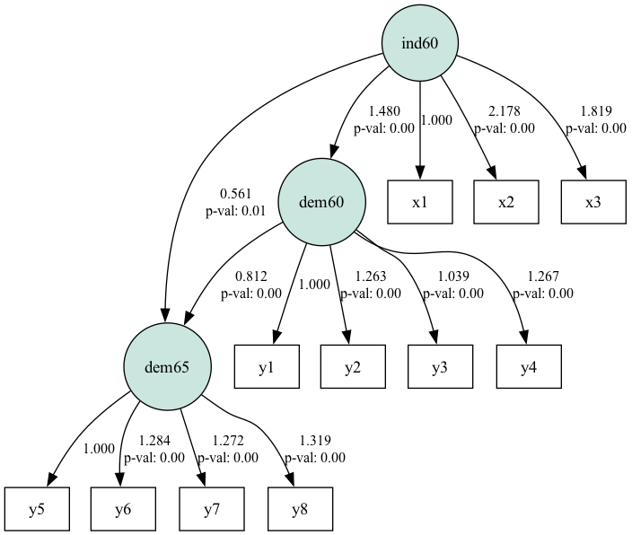
SEM path diagram for political democracy dataset. Source: Image by Author

The diagram shows how the path relates the latent constructs (in circles) and the observed variables. Path coefficients closer to 1 or -1 show strong relationships between variables and those near 0 show weak relationships.

The standard deviations in the table are within the range. Larger values may indicate multicollinearity or model misspecification. The p-values determine the statistical significance of the path coefficients. A p-value less than 0.05 usually indicates that the path is statistically significant. We see 2 cases where the p-value is greater than 0.05. 

All-in-all, the results show that ind60 significantly influences dem60, which, in turn, significantly influences dem65.

Assessing model fit

The hypothesized model should match the observed relationships to assess SEM model fit. Various fit indices are used to assess how well the model fits the data. Here are commonly used ones:

• Chi-Square Test: Compares the observed covariance matrix with the model-implied covariance matrix. A non-significant chi-square indicates a good fit. 
• Root Mean Square Error of Approximation: It evaluates how well the model approximates the data, adjusting for model complexity. Values below 0.05 and up to 0.08 are acceptable.

Common Challenges and Solutions in SEM

Some common challenges of the structural equation modeling technique include the following:

• Non-Normality of Data: SEM generally assumes the data follows a normal distribution. Using non-normal data might affect the standard errors, p-values, and fit indices, leading to unreliable estimates. Data transformation techniques can be applied to normalize the data.
• Missing Data: Complete data is needed for SEM. Missing data can lead to biased results. You can leverage likelihood estimation methods like full information maximum likelihood (FIML) to tackle this.
• Model Fit: When the hypothesized model does not fit the observed data, it leads to misleading interpretations about the relationship between variables. You can make theory-driven adjustments to the model or use modification indices. 

Conclusion

In this article, we reviewed SEM in depth, including its applications, implementation, advantages, and limitations. SEM is a powerful tool for examining complex relationships and causal interactions among observed and latent variables. You should try it out in Python or R for your next analysis project.

If you are interested in the idea of structural equqtion modeling but you prefer R, you can take Structural Equation Modeling with lavaan in R course, which has detailed step-by-step instructions. You can also embark on the Statistician in R career track. If you are committed to Python, read up on the semopy documentation for more use cases of SEM in Python. Finally, if you are interested in advanced Python models that both predict and explain, and exploring ideas of model architecture and feature selection, try our Machine Learning Scientist in Python career track.